Particle Trajectories

Note that the classical equation of motion

\[\vec{F}_i = m_i \frac{\partial \vec{v}_i}{\partial t} = m_i \frac{\partial ^2 r_i}{\partial t^2}\]

is a second order differential equation where the forces are assumed to be constant over the timestep. The usual way of solving this kind of differential equations numerically is by finite difference techniques which involve the use of fixed timestep \({\delta}\)t.

The general idea is to obtain the dynamic information at a later time t + \({\delta}\)t to a significant degree of accuracy, based on the given atomic positions and velocities. This is repeatedly solved on a step-by-step basis and the solution is then propagated through time by using this approximation. The degree of accuracy can be achieved by expanding the Taylor series of expansion about \(\vec{r}(t)\) for an atom i:

\[\vec{r}_i(t+\delta t) = \vec{r}_i(t) + \vec{v}_i(t)\delta t + \frac{1}{2}\vec{a}(t)\delta t^2 + ...\]

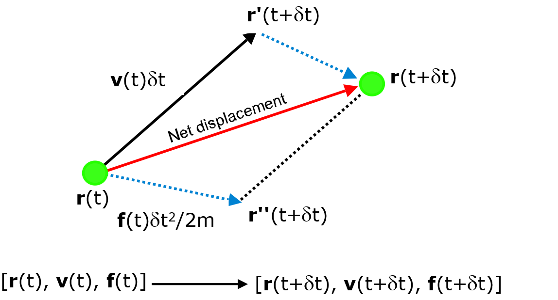
where \(\vec{a}\) is the acceleration, which is \(\frac{\vec{f}}{m}\). Diagram below illustrates the general idea for the integration of motion. Essentially, we are interested to determine the net displacement of an atom over time \({\delta}\)t due to the force experienced by the atom, to produce a new set of dynamic information.

One of the simplest, and fastest to compute is the leapfrog Verlet integration scheme. The scheme requires values of position and force at time t but the velocity at half a timestep behind (t - \(\frac{\delta t}{2}\)).

First of all, the force at time t is computed. Then, the velocity is advanced by t + \(\frac{\delta t}{2}\) using the kinematic equation v = u + ft/m, where m is the mass of the atom:

\[\vec{v}_i (t+\frac{\delta t}{2}) = \vec{v}_i (t-\frac{\delta t}{2}) + (\frac{\vec{f}[\vec{r}_i(t)]\delta t}{m})\]

where the initial velocity (half a step behind) is obtained as

\[\vec{v}_i (t-\frac{\delta t}{2}) = \frac{\vec{r}_i(t) - \vec{r}_i(t-\delta t)}{\delta t}\]

After that, the new position is advanced, or ‘leaped forward’, to a full step t + \({\delta}\)t using the half-step velocity calculated above:

\[\vec{r}_i(t+\delta t) = \vec{r}_i(t) + \vec{v}_i (t+\frac{\delta t}{2})\delta t\]

However, the current velocity at time t would be needed to calculate the properties such as the kinetic and potential energies:

\[\vec{r}_i(t) = \frac{1}{2} [\vec{v}_i (t-\frac{\delta t}{2}) + \vec{v}_i(t+\frac{\delta t}{2})]\]

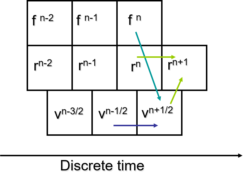
After that, the force at the new position will be calculated and the whole integration process is repeated. Diagram below shows schematic illustration of the integration algorithm.

Note that, although verlet leap frog is simple and faster than most other schemes, it is not time reversible and become unstable over long time scales. The use of a symplectic integrator provides time reversibility and long-term stability. One commonly-used integration scheme for MD simulations is Velocity Verlet (VV), which is second-order accurate (i.e. errors are proportional to the square of the timestep size \({\delta}\)t) and updates particle positions and velocities without requiring additional memory to do so. Please refer to DL_POLY manual for details about VV scheme.

Note

By default, DL_POLY offers the VV. It generates trajectories in the microcanonical (NVE) ensemble in which the total energy is conserved. If this drifts or fluctuates excessively in the course of a simulation, this may mean the timestep is too large or the potential cutoffs are too small.

^ GO TO TOP ^