Lattice Boltzmann Equation (LBE)
Summary
The Lattice Boltzmann Equation (LBE) is a mesoscale modelling method with a statistical mechanics approach. Rather than tracking the motion of individual particles, distribution functions are defined to describe the probability of finding particles at a given point in time and space with a particular momentum. The distribution functions evolve over time by considering how the particles collide and subsequently move. Summing their moments over all possible particle momenta gives macroscopic properties such as fluid density and momentum. Confining the particles to a grid and to preset links between grid points simplifies the calculations but still provides enough information to correctly calculate hydrodynamic behaviour.
The particles in LBE can be considered flexibly, thus allowing larger length and time scales than atomistic modelling methods while still incorporating some detail of molecular interactions. Boundary conditions can be treated in intuitive and simple ways, allowing systems with complex geometries to be modelled nearly as efficiently as simpler ones. Methods to allow multiple fluids and phases to be modelled in LBE without fundamentally changing the algorithm have also been devised, as have ways to represent fluids with non-standard rheological behaviour and to incorporate diffusion and heat transfer effects.
Background
LBE can be considered as a variant form of lattice gas cellular automata (LGCA), a modelling method that directly models particles colliding and moving around a regular grid [1]. By replacing binary particle occupation numbers with probability distribution functions [Frisch1987], several of LGCA’s shortcomings as a method to model fluid flows (e.g. noise, lack of Galilean invariance) were overcome.
Given a lattice link \(i\) with vector (and momentum) \(\mathbf{e}_i\), we can define an associated distribution function \(f_i\) for each grid point. The distribution functions evolve via the following equation:
where \(C_i\) is a collision operator for link \(i\) that may depend upon all distribution functions at a given grid point \(\mathbf{x}\). The evolution equation (1) can be also expressed by separating out the collision and propagation stages as (2) and (3) respectively:
The collision operator \(C_i\) can take several different forms, but the simplest and most common form without considering forces acting on the fluid is based on the Bhatnagar-Gross-Krook (BGK) approximation. This uses a single relaxation time \(\tau\) as the parameter defining the timescale of collisions [Qian1992]:
where \(f_i^{eq}\) is a distribution function corresponding to a local equilibrium state [2]. This local equilibrium distribution function is available as a function of macroscopic fluid density and velocity, usually of the form for mildly compressible fluids at speeds significantly lower than the speed of sound \(c_s\):
where \(w_i\) is a weighting parameter dependent on link and lattice scheme. To use (5) in the collision operator given in (4), we can calculate the macroscopic density and velocity by finding the zeroth and first moments of the distribution functions:
It is ultimately possible - using a lot of mathematics(!) - to show that the above equations can accurately represent fluid flow by assuming the majority of distribution functions come from local equilibrium values and their non-equilibrium parts scale with the Knudsen number \(Kn\) (ratio of molecular mean free path to molecular length scale). By expanding (1) about \(Kn\) in time and space, applying a Chapman-Enskog expansion to various time and length scales, separating out the resulting equations based on orders of \(Kn\) and summing over all lattice links, we can eventually obtain conservation equations for mass and momentum. These conservation equations lead to the Navier-Stokes equations for systems with small variations in density [Chen1998], i.e.
from which we can define the speed of sound for the LBE fluid:
the equation of state:
and a relationship between kinematic viscosity (ratio of dynamic viscosity and density) and the relaxation time:
We can select a value of \(\tau\) to avoid numerical instabilities in LBE simulations (i.e. not too close to \(\frac{1}{2}\)). Along with the kinematic viscosity and speed of sound for a given fluid, this sets the length scale (lattice spacing \(\Delta x\)) and time scale (timestep \(\Delta t\)) [3]. We typically have free choice over density values used in LBE simulations, although keeping it around 1 can help maximise the calculation precision we have available.
Extensions
We can include additional fluids by either modelling them in separate lattices and calculating interaction forces between them - which we can then apply as an additional part of the collision operator - or by modifying (5) to obtain the correct free energy density function and apply interfacial tensions. These approaches allow us to model immiscible fluids, including drops suspended in background fluids that can represent e.g. fluid-filled vesicles or cell membranes.
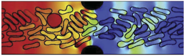
LBE simulation of non-spherical fluid-filled vesicles flowing through a constricted channel [Montessori2018].
Alternative forms of (5) can be used to represent completely incompressible fluids and diffusive processes: the latter can represent diffusion of solutes or heat transfers and can be coupled to bulk fluid flows. We can also calculate shear rates locally at each grid point and use these to determine local values of viscosity according to a given rheological model for non-Newtonian fluids such as blood.
Boundary conditions are defined to specify missing distribution functions ‘re-entering’ the system and are used to obtain required fluid densities and/or velocities. The simplest form of boundary condition we can use is bounce back, where a boundary grid point reflects distribution functions entering it: this has the effect of applying a no-slip condition (i.e. zero velocity) at any arbitrary boundary point without any extensive calculations. It is therefore straightforward and computationally inexpensive to use LBE for flows in porous media or past complex shapes.
Footnotes
| [1] | This is the same modelling method that was modified to produce Dissipative Particle Dynamics (DPD) [Hoogerbrugge1992]! |
| [2] | An interpretation of (4) states that the collision pushes the system towards an equilibrium state and \(\tau\) determines how quickly this occurs. |
| [3] | For example, if we want to model water at room temperature (298 K), its speed of sound is 1498 m s -1 and kinematic viscosity is \(10^{-6}\) m s -2. If we select a relaxation time of \(\tau = 1\), this sets the lattice spacing as \(\Delta x = \frac{\sqrt{3} \nu}{c_s \left(\tau - \frac{1}{2}\right)} \approx 2.3125 \times 10^{-9}\) m and the timestep as \(\Delta t = \frac{\nu}{c_s^2 \left(\tau - \frac{1}{2}\right)} \approx 8.9126 \times 10^{-13}\) s. |
References
| [Frisch1987] | U Frisch, B Hasslacher, P Lallemand, Y Pomeau and JP Rivet, Lattice gas hydrodynamics in two and three dimensions, Complex Systems, 1, 649-707, 1987. |
| [Qian1992] | YH Qian, D d’Humières and P Lallemand, Lattice BGK models for Navier-Stokes equation, EPL, 17, 479-484, 1992, doi: 10.1209/0295-5075/17/6/001. |
| [Chen1998] | S Chen and GD Doolen, Lattice Boltzmann Method for fluid flows, Annual Review of Fluid Mechanics, 30, 329-364, 1998, doi: 10.1146/annurev.fluid.30.1.329. |
| [Montessori2018] | A Montessori, I Halliday, M Lauricella, SV Lishchuk, G Pontrelli, TJ Spencer and S Succi, ‘Multicomponent lattice Boltzmann models for biological applications’, Chapter 20 in Numerical methods and advanced simulation in biomechanics and biological processes (ed. M Cerrolaza, SJ Shefelbine and D Garzón-Alvarado), pp. 357-370, Academic Press, Elsevier, 2018. |