Simulation Run

Step 1: If you have not yet done so, obtain and compile DL_MESO, specifically DL_MESO_DPD and the utilities. If you have an implementation of MPI on your machine, the parallel version of DL_MESO_DPD is highly recommended; otherwise compile the serial version (using the makefile dl_meso/DPD/makefiles/Makefile-serial).

TIP:If you are using a high-performance computing (HPC) facility, it might have a pre-compiled DL_MESO module that you can load in and use, which should make the required executable files available to you when submitting a job. If it does not, you can still compile DL_MESO_DPD yourself using the instructions linked above, although you may need to consult the HPC facility’s documentation to find out how to load in compilers and MPI.

Step 2: Select your working folder, which can either be the dl_meso/WORK folder - where the DL_MESO and utility executables were created - or another folder of your choosing. If the latter, either copy the dpd.exe and other executable files (ending .exe) into that folder or work out the path to the dl_meso/WORK folder from that folder (e.g. use the command pwd to provide the absolute path).

Copy the CONTROL and FIELD files into your working folder.

TIP:The DL_MESO_DPD executable (dpd.exe) expects the CONTROL and FIELD input files to be in the same directory where it is launched, and needs to find these files to run a simulation successfully.

Step 3: Navigate a terminal (command line) window into the working folder and either type

./dpd.exe

to run the serial version of DL_MESO_DPD in that folder, or

mpirun -np X ./dpd.exe

to run the parallel version, substituting X with the required number of processor cores. If the dpd.exe executable is in a different folder, replace the dot in either command with the path to the dl_meso/WORK folder, e.g.

/path/to/dl_meso/WORK/dpd.exe
mpirun -np X /path/to/dl_meso/WORK/dpd.exe

If you are using a high-performance computing (HPC) service with a batch job manager (e.g. Slurm), you will need to write a job script to specify the computing resources (number of cores, runtime) and the mpirun (or similar) command, which would be used to submit the calculation to a job queue. The form this job script should take and how to use it will depend on the HPC system in use, so you will need to consult its documentation for further details.

A number of files will be generated during the run, including an OUTPUT file describing the progression of the simulation, export and REVIVE files to enable simulation restart, a CORREL file with tabulated system properties and a HISTORY file with particle trajectories.

The images below show the contents of the OUTPUT file for the simple fluid example.

This first image shows the point at which equilibration has finished and the sample period has begun, and reports instantaneous (first line for each given timestep) and rolling-average (second line) values for system-wide properties (e.g. energies per particle, pressure, temperature).

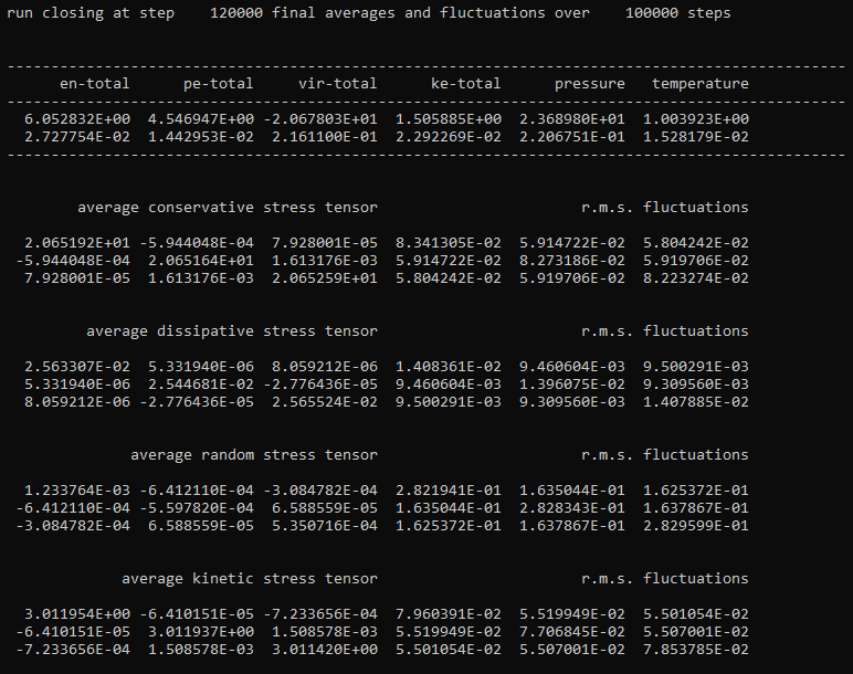
The second image shows part of the summary written to the OUTPUT file once the calculation has finished, including average values and fluctuations (standard deviations) of system properties, including pressure tensors separated into four contributions, which are calculated during the simulation after equilibration.

Step 4: Take a look at the values of system properties in the OUTPUT file (or the CORREL file) and check they are settling around average values after equilibration has taken place.

For a constant-volume (NVT) ensemble, the total potential energy per particle (pe-total) and system pressure should settle and oscillate around average values, indicating the system is likely to have reached an equilibrium state. In the example shown here (for a simple fluid), the potential energy per particle after equilibration is reported as \(4.547 \pm 0.014\), which is markedly different from the value at the start of the simulation (\(3.837\)), while the pressure is reported as \(23.69 \pm 0.22\). Both the potential energy and the system pressure are configurational properties, i.e. they depend on the positions or arrangements of particles in the system.

The system temperature for this static system (i.e. one with no applied flow field) should also settle and oscillate around an average value close to the temperature specified in the CONTROL file. In this case, the temperature is reported as \(1.004 \pm 0.015\). This kinetic property is dependent on particle velocities and should be controlled by the DPD thermostat (dissipative and random forces) in this instance.

The instantaneous values of these properties at each reported timestep can be checked against rolling average values, which sample the properties over a number of previous timesteps, to check whether or not the system is still moving towards an equilibrated state.

Step 5: If the system properties have not yet settled and an equilibrium state has not yet been reached, the simulation can be extended further to give it more time to equilibrate. This can be achieved in DL_MESO_DPD without re-calculating previous timesteps by restarting the simulation.

Open the CONTROL file, increase the total number of timesteps (steps) and add the following line before the final finish directive:

restart

before running DL_MESO_DPD again (Step 3).

Restarting DL_MESO_DPD requires an export file, which includes the system configuration (bead positions, velocities and forces) and is (over)written periodically by DL_MESO_DPD during a calculation.

Resuming a previous calculation from exactly where it left off additionally requires a REVIVE file, which is also generated periodically by DL_MESO_DPD during a calculation and contains statistical accumulators and random number generator states.

To start a new calculation without using the statistical accumulators in the REVIVE file, use the following line in the CONTROL file:

restart noscale

which uses the state in the export file as the initial configuration for the new calculation. If the system temperature was very far away from the required value, use

restart scale

in the CONTROL file, which will also rescale the particle velocities in the export file to provide the correct temperature at the start of the calculation.

Step 6 (optional): To look at non-equilibrium hydrodynamic properties (e.g. viscosity), a linear shear flow with a constant velocity gradient can be applied to the simulation using Lees-Edwards periodic boundary conditions.

Open the CONTROL file and add the following line before finish:

surface shear y 20000

which tells DL_MESO_DPD to apply shear orthogonally to the y-axis, starting from timestep number 20000 (the number of equilibration timesteps). For analysis of this system, change the number at the end of the trajectory line from 0 to 1, e.g.

trajectory 100000 100 1

to include particle velocities in the HISTORY trajectory file. You may also wish to start sampling trajectories later to allow the system to settle to a steady-state and increase the sampling frequency.

Open the FIELD file and add the following two lines before close:

EXTERNAL
shear  1.0  0.0  0.0

which applies a velocity of \((1.0, 0.0, 0.0)\) (i.e. 1.0 in the x-direction) at the top wall and \((-1.0, 0.0, 0.0)\) at the bottom wall.

TIPS:The wall velocities need to be sufficiently high for the shearing to be detected over the thermal motion (internal energy) of the beads, which sets a minimum shear rate (velocity gradient) for these simulations.

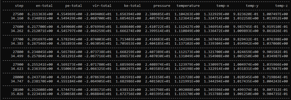
For systems with external flow fields, the OUTPUT file will include partial temperatures in each Cartesian direction, shown as temp-x, temp-y and temp-z in the above example for the simple fluid.

Both the system temperature and the partial temperature(s) for the Cartesian component(s) in which the shear is applied (in this case, the x-direction) will end up higher than the temperature specified in the CONTROL file due to the resulting flow field, but both properties should average out to constant values. The partial temperatures in other Cartesian directions (y- and z-directions) should not be affected by the flow field and therefore should settle to and oscillate around the value specified in CONTROL.