Analysing Results

The results from a DL_MESO_DPD simulation include system-wide properties obtained during the DPD calculation found in OUTPUT and CORREL files and particle trajectories in the HISTORY file. As well as visualising the simulation, the trajectories can be used to analyse it further by calculating additional configurational and kinetic properties. Some system properties that can frequently be calculated from DPD simulations include radial distribution functions (RDFs), mean squared displacements (MSDs) and shear viscosities.

Various utilities are included with DL_MESO that enable the user to process the HISTORY file generated by a DL_MESO_DPD calculation, which can be compiled according to the instructions in the Ready, get set, go guide. Alternatively, Python scripts are available to carry out the processing and plot some of the results. The analysis scripts require a module to read HISTORY files (dlmhistoryread.py).

TIP:To display the available command-line options for a utility or an analysis script, run it with the option -h (e.g. ./rdf.exe -h. Using this option will not run any analysis.

The results in the CORREL file and those derived from the HISTORY file using utilities or scripts are given in text files mainly as columns of numbers: the exact format will depend on the file and/or the property being examined. These data can be visualised either by using graphing software such as Gnuplot, a spreadsheet program (after importing the file) or by using the DL_MESO_DPD Result Viewer (dlmresultviewer.py) Python script. The Result Viewer is a graphical interface program that uses Qt and a Python language interface (PyQt5), both of which can be installed using Python’s package installer, e.g.:

pip install pyqt5

TIP:Some Python 3 installations may use pip3 instead of pip for the installer and python3 in place of python to run scripts or the interpreter.

Other Python packages (docopt, numpy, scipy, matplotlib and numba) may also need to be installed to run the analysis scripts and the Result Viewer. If any of these are missing as indicated in any error messages when trying to run a script, they can be installed using a similar command to the one above.

Statistical properties (energies, temperature, pressure etc.):

The CORREL file consists of columns of system-wide properties at user-specified intervals in time during the DL_MESO_DPD calculation, starting from the end of any equilibration period. The properties can include energies per particle (including potential energies split into different contributions, e.g. bonds, electrostatics), pressure, pressure tensors, temperature, volume, bond lengths, angles and dihedrals. The number of columns of data will depend upon the contents of the simulation and its interactions, but the first column will always be time in DPD units.

The tabulated data can be visualised as a graphical plot using Gnuplot by launching the program in a terminal window from the directory with the CORREL file:

gnuplot

and then typing a command specifying the file and the columns for the x- and y-axes, e.g.

plot 'CORREL' u 1:3 w li

will plot the potential energy per particle (column 3) as a function of time (column 1) and display the data as a line plot. Other commands are available in Gnuplot to analyse the available data points, e.g.

stats 'CORREL' u 1:3 w li

which will calculate and display time-averaged values, standard deviations etc.

TIP:It is worth taking a look at the beginning of the CORREL file in a text editor and making a note of which columns consist of which properties before opening it in Gnuplot. The first line of the file includes labels for each column, which are ignored by Gnuplot.

Alternatively, the DL_MESO_DPD Result Viewer can read the file when launched:

python dlmresultviewer.py

which opens a window with a graph plotter and a pull-down box to select the property to be plotted as a function of time, which is populated automatically based on the contents of the CORREL file. There are also options to plot histograms, running averages, autocorrelation functions and Fourier transforms for each property.

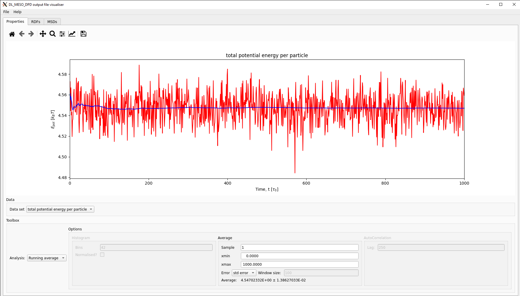
For most DPD simulations (i.e. those without applied flows), these properties should be checked to ensure the system has indeed reached equilibrium (as mentioned for the Simulation Run) and therefore their values can be regarded as representative. For instance, the potential energy per particle should reach a minimum (averaged) value and oscillate around it, while the system temperature should oscillate around the value specified in the CONTROL file. The property likely to require the longest simulation runtime (largest number of timesteps) to settle is the system pressure, as this depends on both the potential (Hamiltonian) and the system kinetics (shown by e.g. temperature).

Simulations involving flow fields do not formally reach an equilibrium state, but most should reach a steady-state with constant values for both potential and kinetic properties. Since the system temperature is often calculated from kinetic energy, applying a flow field can result in a higher-than-expected temperature. However, if the flow is only applied in one direction along a Cartesian axis, partial temperatures for other dimensions should still settle to the value specified for the simulation.

Radial distribution functions:

There are two options for obtaining RDFs from DL_MESO_DPD HISTORY files:

• The utility rdf.exe supplied with DL_MESO, or
• The Python script history_dlm_to_rdf.py

Both of these will calculate all RDFs between available particle types, including the RDF between beads of all types, and write these to a RDFDAT file, using up to all of the available trajectory frames in a HISTORY file.

To use the utility, type:

./rdf.exe -d 0.02 -c 3.0

or to use the script, type:

python history_dlm_to_rdf.py --dr 0.02 --rcut 3.0

where 0.02 is the suggested distance spacing between histogram bins and 3.0 is the suggested maximum distance between particle pairs. The size of the distance spacing should strike a balance between memory requirements for binning (smaller values require more bins) and ensuring localised features in a radial distribution function are not smeared out. The maximum (cutoff) distance between particle pairs also has an effect on the memory requirements for binning, but this should be sufficiently large to observe convergence at longer distances than the interaction cutoffs used in DPD calculations: due to periodic boundary conditions, it cannot be more than half the length of the box.

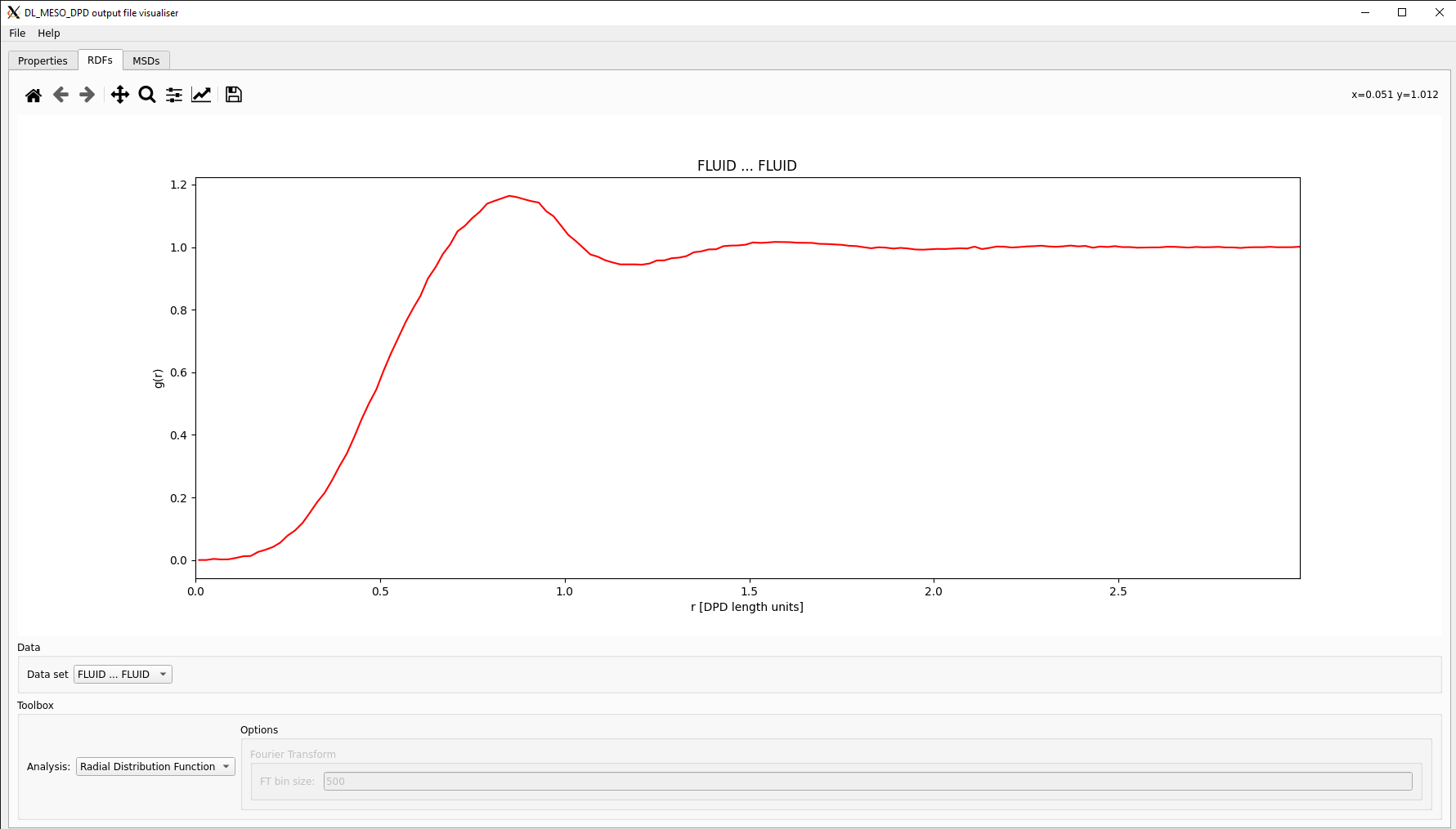
Both the utility and the script end up producing an RDFDAT file, which is formatted to enable the RDFs for all species pairs and the RDF for all particles to be plotted separately. Each data block consists of three columns: distance \(r\), (given as middle values for each histogram bin), the value of RDF for the species pair \(g(r)\) and the sum (integral) of RDF from zero to \(r\).

The RDFDAT file can be opened and imported into a spreadsheet program as a fixed-width text file. Alternatively, if you know which data block in the file you wish to plot in Gnuplot, you can select the block in the command line, e.g. for the first block

plot 'RDFDAT' index 1 u 1:2 w li

The DL_MESO_DPD Result Viewer can also read the RDFDAT file and plot the RDFs, which can be selected using a drop-down box. This visualisation script can also calculate and plot structure factors, which are based on Fourier transforms of RDFs. The RDF calculation utility and script can also calculate structure factors and write them to RDFFFT files which are similarly formatted to RDFDAT, although the Result Viewer cannot read these.

Mean squared displacements and diffusivity:

Two options are available to obtain MSDs from DL_MESO_DPD HISTORY files:

• The utility msd.exe supplied with DL_MESO (version 2.8 and later), or
• The Python script history_dlm_to_msd.py

Both of these will calculate MSDs for all available particle types, including the MSD for all bead types, and write these to a MSDDAT file, using up to all of the available trajectory frames in a HISTORY file. They will also calculate estimates for the self-diffusivity of each bead type and for the entire system by sampling gradients of the MSDs.

To use the utility, type:

./msd.exe

or to use the script, type:

python history_dlm_to_msd.py

There are command-line options available to specify the number of trajectory frames over which to find gradients of MSDs for diffusivity calculations (-ba for the utility, --block for the script), although the default value of 10 is normally adequate. The utility and script both assume particles move less than half a minimum box size (\(L_{min}\)) between each frame in the HISTORY file, which sets a maximum time between frames of around \(\frac{L_{min}}{2}\sqrt{\frac{m}{3k_B T}}\) to calculate MSDs reliably.

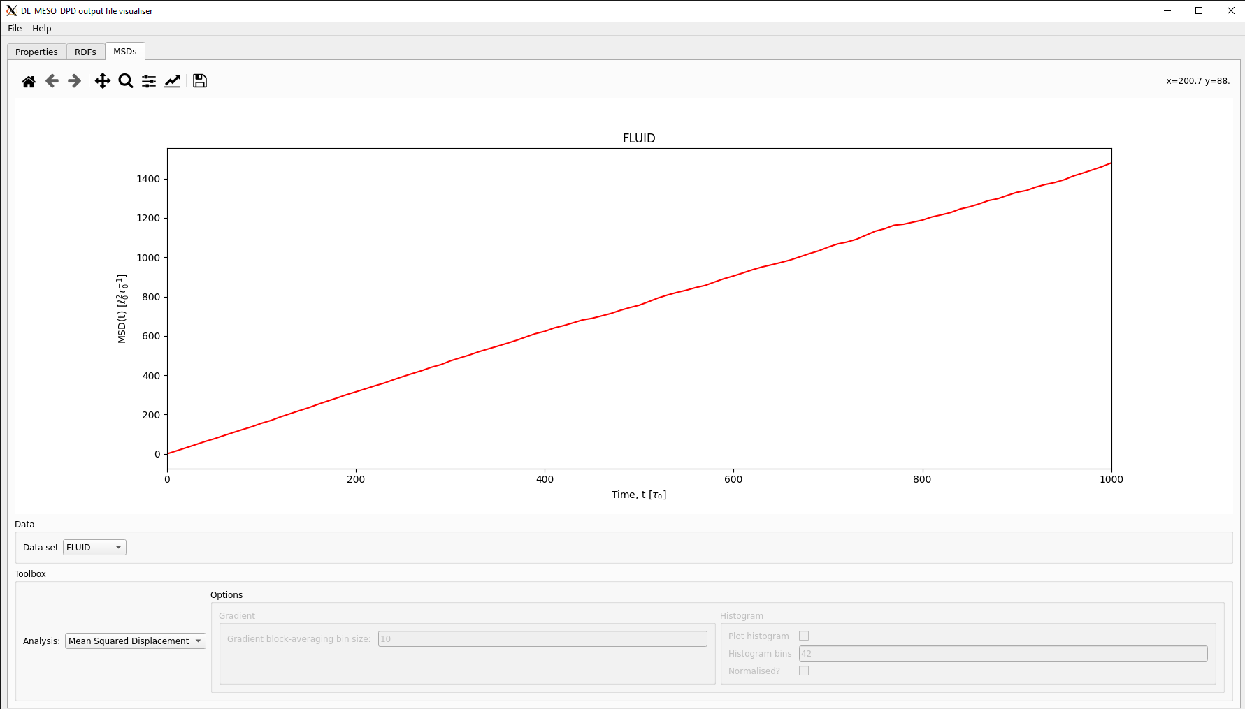
Both the utility and the script end up producing an MSDDAT file, which is formatted to enable the MSDs for all species (given in the same order as the FIELD file used for the simulation) and for all particles to be plotted separately. Each data block consists of three columns: time \(t\), the value of MSD for the species at time \(t\) and the square root of the MSD (the root mean squared displacement). They will also print mean values for the self-diffusivities and standard deviations (given as possible errors) for each and all species based on calculating gradients of the MSDs.

The MSDDAT file can be opened and imported into a spreadsheet program as a fixed-width text file. Alternatively, if you know which data block in the file you wish to plot in Gnuplot, you can select it in the command line, e.g. for the first block (corresponding to the first particle species)

plot 'MSDDAT' index 1 u 1:2 w li

The DL_MESO_DPD Result Viewer can also read the MSDDAT file and plot the MSDs, which can be selected using a drop-down box. This visualisation script can also calculate and plot diffusivities by calculating gradients over a set number of points: these can be plotted either as a function of time or as a distribution with histograms.

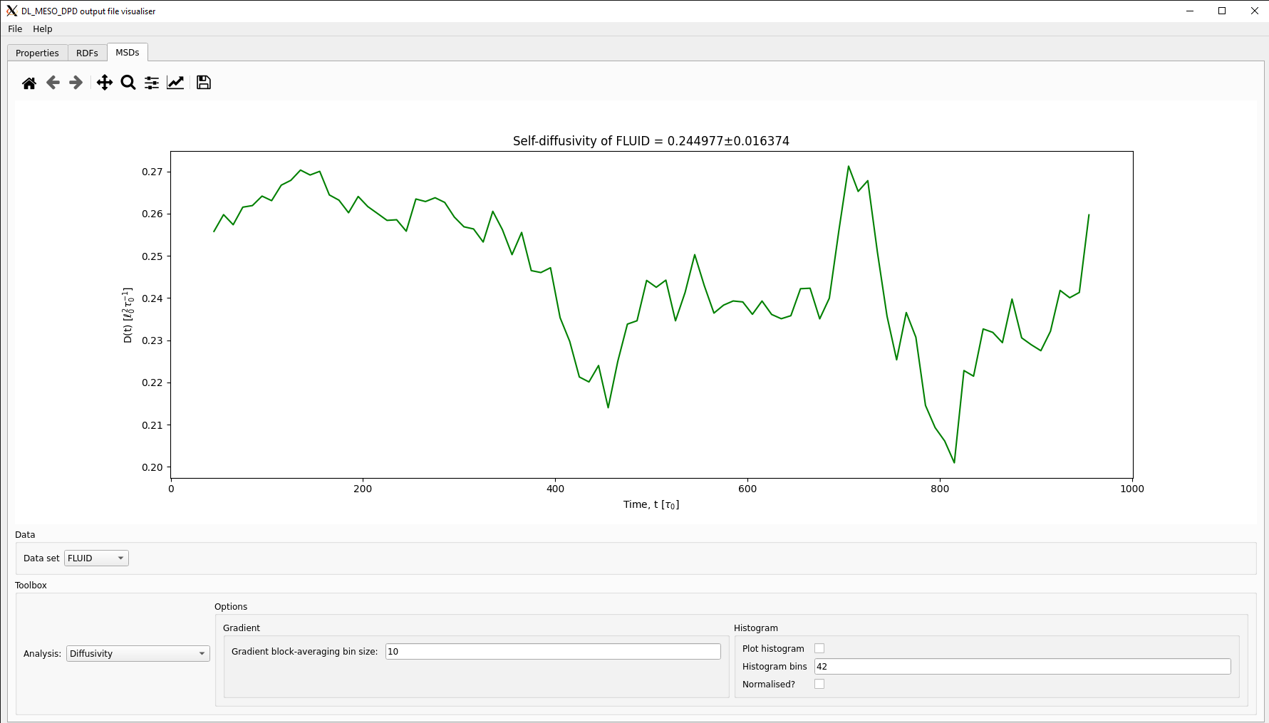
The self-diffusivity shown here for the simple fluid (\(D = 0.245 \pm 0.016\)) can be used to determine the DPD time unit \(\tau_0\), assuming each bead consists of one molecule of water at room temperature \(T = 298\) K (\(N_w = 1\), \(D_w = 2.299 \times 10^{-9}\) m\(^{2}\) s\(^{-1}\), \(r_c = 4.48 \times 10^{-10}\) m):

\[\tau_0 = \frac{N_m D_{sim} r_c^2}{D_w} = \frac{0.245 \left(4.48 \times 10^{-10} \right)^2}{2.299 \times 10^{-9}} \text{ s} \approx 2.14 \times 10^{-11} \text{ s}.\]

Viscosity:

For a DL_MESO_DPD simulation with an applied linear shear flow, the shear stress can be calculated from the pressure tensor, which can be obtained either from the CORREL file or at the end of the OUTPUT file (combining together the potential, dissipative, random and kinetic contributions).

TIP:While the pressure tensor in the OUTPUT file is easiest to read as it provides averaged values and fluctuations (to estimate statistical errors), it is only likely to be representative if the system has reached a steady state before DL_MESO_DPD starts sampling the tensor (i.e. after equilibration). The CORREL file enables the range of values to be selected to omit those during equilibration and the establishment of shear flow.

To verify the correct velocity gradient has been achieved and is constant, a time-averaged velocity profile can be obtained from the DL_MESO_DPD HISTORY file using either:

• The utility local.exe supplied with DL_MESO, or
• The Python script history_dlm_to_local_vtk.py

Both of these will divide the simulation box into cuboids or slices and calculate localised properties for each section based on the available particle data in the HISTORY file, i.e. positions, velocities and forces. The properties can include particle densities, velocities, temperatures (including partial values for each Cartesian direction) and pressure tensors. These data are written to VTK-formatted files, one for each trajectory frame and an additional file for time-averaged values of the properties. (The utility will produce these files in a legacy VTK format ending with .vtk, while the script produces files in an XML format ending with .vts.)

To use the utility, type:

./local.exe -nx 1 -ny 100 -nz 1

or to use the script, type:

python history_dlm_to_local_vtk.py --nx 1 --ny 100 --nz 1

which splits the box into 100 slices in the \(y\)-direction without dividing the box up in the \(x\)- and \(y\)-directions. If you are not interested in instantaneous values for each trajectory frame, you can add an additional command-line option (-av for the utility, --averageonly for the script) to solely write the time-averaged data.

TIP:The VTK files with instantaneous values calculated for each individual trajectory frame are likely to be statistically noisy. While these can help gauge how well a simulation has run and give time progression for the localised properties, they are unlikely to be usable for providing representative values: at least some time-averaging will be needed, even when the system has reached equilibrium.

The resulting VTK files can be opened in ParaView and visualised as grid-based data. Filters can be applied to manipulate the data and plot along selected lines, including one placed orthogonally to shearing boundaries.

The DL_MESO_DPD Result viewer can also read the VTK file with time-averaged properties (averages.vtk or averages.vts) and plot lines for each calculated property along a Cartesian direction selected by the user using a pull-down box. If the box has been split in other directions, the user can use sliders to select the cell tangential to the line, although the viewer will choose the central one by default when it starts. A line representing a best fit to a selected polynomial function can also be drawn, with the function displayed at the top of the graph.

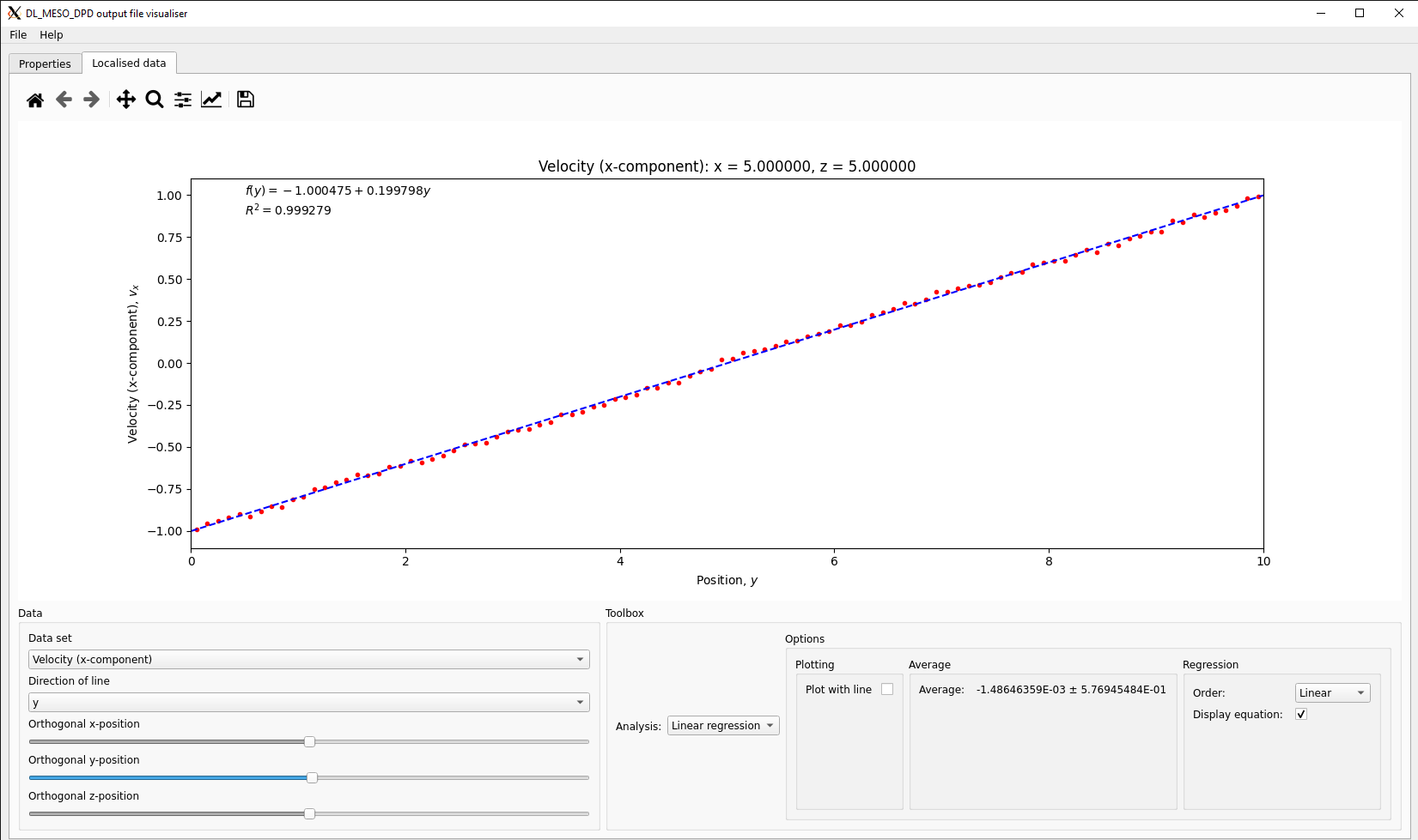
In the case shown above for the simple fluid, the plot of the \(x\)-component of velocity along the \(y\)-direction gives a linear velocity profile. The function fitted to this data gives a velocity gradient (shear rate) of \(0.1998~\tau_0^{-1}\), very close to the intended value of \(0.2~\tau_0^{-1}\). Along with the \(yx\)-component of pressure tensor \(p_{yx} = -0.1903~k_B T~r_c^{-3}\), this leads to a dynamic viscosity of \(\mu \approx 0.952~k_B T\tau_0~r_c^{-3}\). The kinematic viscosity is equal to this value divided by the mass density \(m\rho\), i.e. \(\nu \approx 0.317~r_c^{2}~\tau_0^{-1}\).

TIP:While it is possible to calculate a single viscosity value using the above approach, you might want to try further simulations with different velocity gradients (shear rates) to see how the viscosity might vary. A plot of shear stress as a function of shear rate will provide detailed rheological behaviour of the material being studied.