Analysing Results

The main results from a DL_MESO_LBE simulation are snapshots taken at periodic intervals given in VTK files, and the total masses and momenta of the fluids at those same points in time given on the screen or in the standard output. As well as visualising the simulation, the snapshots can be used to analyse it further by calculating (and visualising) other properties.

ParaView can be used to visualise and calculate certain properties for each snapshot generated by a DL_MESO_LBE calculation. These include graphs that can be viewed in ParaView itself: the values used for these plots can be exported to text files to visualise later using graphing software such as Gnuplot or a spreadsheet program after importing the file. Alternatively, a Python script specific to the simulations given here is available to work out certain properties.

TIP:To display the available command-line options for an analysis script, run it with the option -h (e.g. python vtk_to_twophase.py -h. Using this option will not run any analysis.

Other Python packages (docopt, numpy, scipy, matplotlib and scikit-image) may also need to be installed to run the analysis scripts. If any of these are missing as indicated in any error messages when trying to run a script, they can be installed using Python’s package installer, e.g. :

pip install docopt

Some Python 3 installations may use pip3 instead of pip for the installer and python3 in place of python to run scripts or the interpreter.

Equilibrium densities of vapour and liquid phases:

By the end of the DL_MESO_LBE calculations of our fluid (hydrogen chloride), it should have separated into two phases: one at a lower density that we can consider as vapour, and a higher density one that is liquid. You can check this has happened simply by opening the VTK files in ParaView and playing through the calculation.

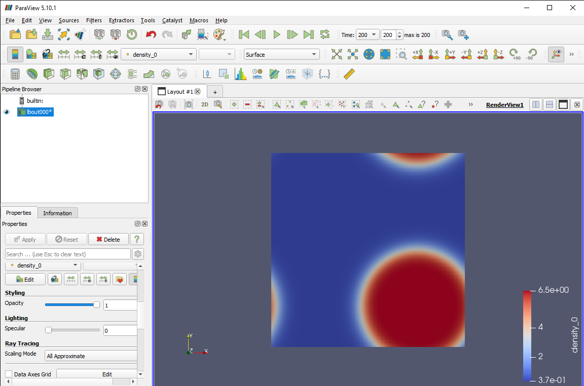
The example above for the simulation with Shan-Chen pseudopotential interactions shows that the fluid has separated into a liquid drop surrounded by vapour. The colour scale indicates the minimum and maximum densities found on the grid, which are also available inside the Information tab. These indicate that the vapour density \(\rho_v \approx 0.3669\) and the liquid density \(\rho_l \approx 6.5017\).

While not shown here, the equivalent densities from the free-energy calculation are \(\rho_v \approx 0.4878\) and \(\rho_l \approx 6.2784\). Note that a Maxwell construction carried out by the maxwell.py script predicts \(\rho_v \approx 0.3955\) and \(\rho_l \approx 6.4471\).

Spurious microcurrents:

A consequence of how the fluid interactions are implemented in multiple-phase LBE simulations are spurious flows (microcurrents) generated at the interface between the phases. The magnitude of these microcurrents can affect the ability of a simulation to attain numerical stability and obtain an equilibrium state. This can be a particular problem for lower system temperatures and/or systems with flow fields: the microcurrents can limit the density contrast (ratio of liquid to vapour densities) that can be obtained.

To obtain a measure of the microcurrents for each simulation, you can visualise the velocity magnitudes in ParaView by using the pull-down boxes to select the property and, for vector properties such as velocity, magnitude (here giving the speed) and Cartesian coordinates.

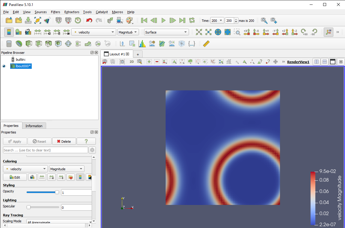
Plot of velocity magnitudes (speeds) for Shan-Chen calculation

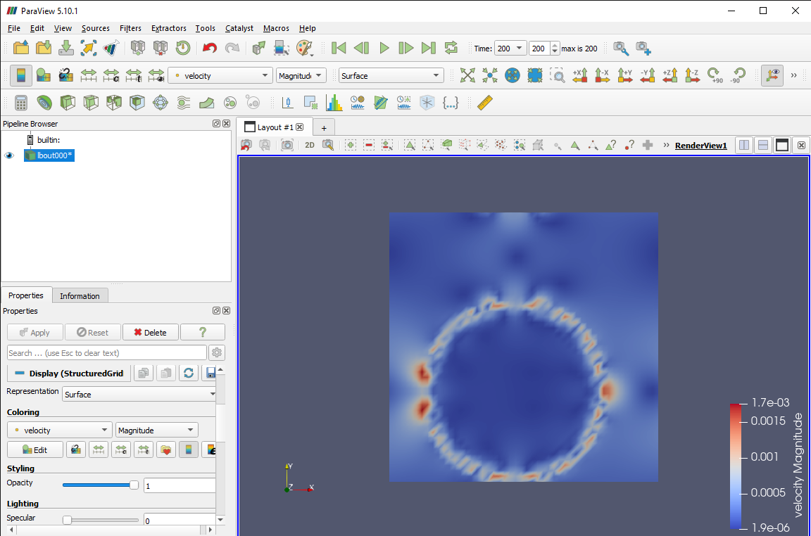
Plot of velocity magnitudes (speeds) for free-energy calculation

The maximum fluid speed in the Shan-Chen simulation is around \(0.0955 \frac{\Delta x}{\Delta t}\), while for the free-energy calculation it is around \(0.0017 \frac{\Delta x}{\Delta t}\). Note that the maximum speeds can be found in regions corresponding to the interface between the two phases, where the densities have intermediate values between those for the bulk vapour and liquid.

TIP:It is possible to extend the range of density contrasts for both methods by reducing the magnitudes of microcurrents. One approach to do this is to reduce the values of \(R\) and \(a\) by a common factor [Liu2010]: this reduces the density or pseudopotential gradients (and thus Shan-Chen forces) but also widens the interfacial region. We can also use more complex collisions (e.g. multiple-relaxation-time, MRT) with additional parameters to reduce numerical instabilities in the LBE calculations.

Drop size:

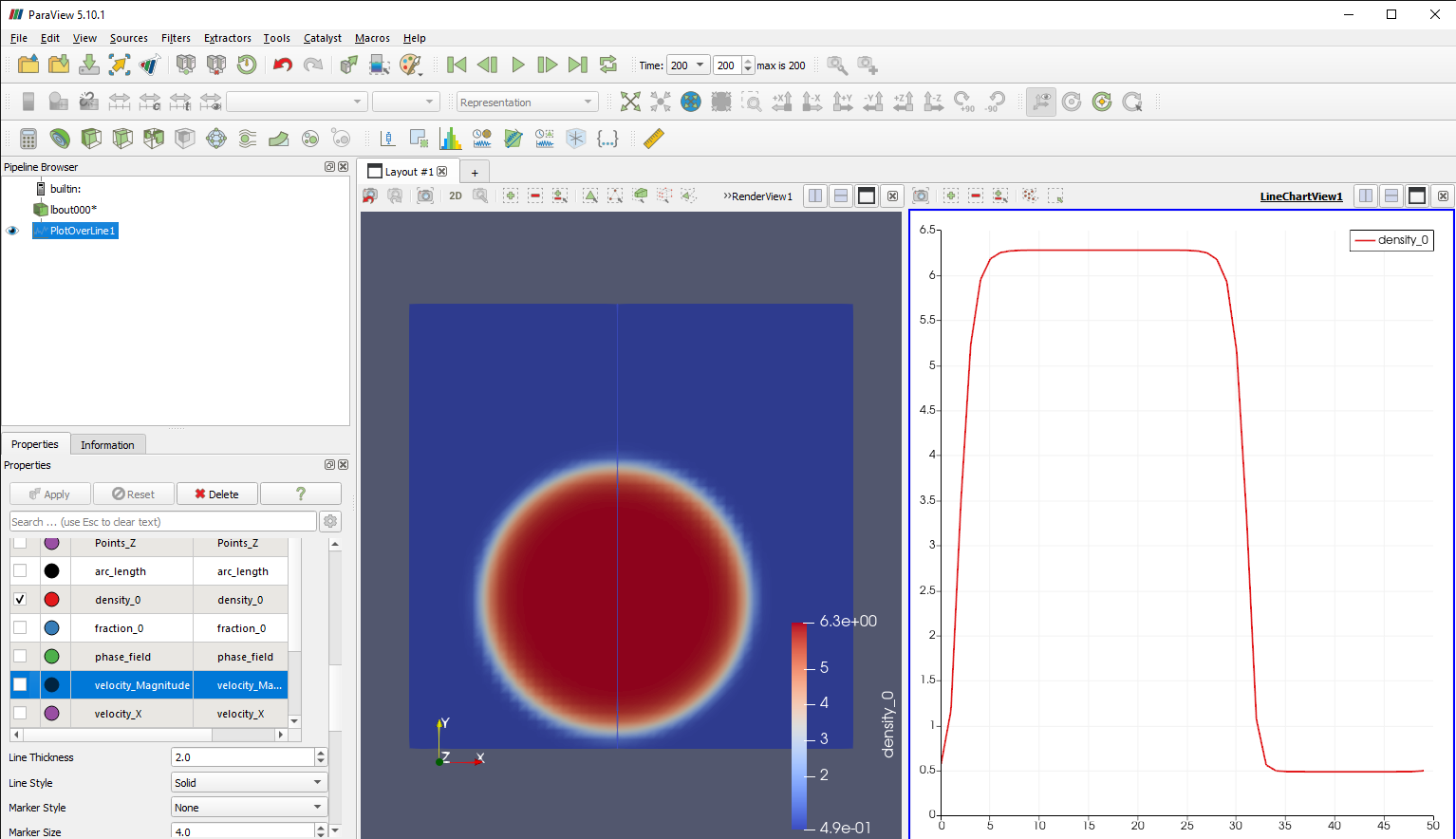
The Plot Over Line filter in ParaView can be used to look at the density profile through the liquid drop and the bulk vapour phase outside it. Note that the change in density from vapour to liquid (or vice versa) is not abrupt or stepwise, but involves a more gradual change over a short distance in the form of a hyperbolic tangent function.

TIP:To save the data used for the plot, select Save Data from the File menu and choose Comma or Tab Delimited Files as the file type, as well as a filename. The resulting file can then be opened in a spreadsheet program (e.g. Excel) or plotting software (e.g. Gnuplot), noting that the distance along the line is given as arc_length.

To determine the size (radius or diameter) of the drop, we can define a phase index:

\[\rho^N = \frac{\rho - \rho_v}{\rho_l - \rho_v}\]

using the values of bulk vapour and liquid densities, \(\rho_v\) and \(\rho_l\), as determined above. The value of this index will ordinarily vary between 0 for pure vapour and 1 for pure liquid, while the interfacial region will have intermediate values. The centre of mass for the drop can be determined by summing moments of the phase index, e.g.

\[\mathbf{X} = \frac{\sum_{i} \rho^N (\mathbf{x}_i) \mathbf{x}_i}{\sum_{i} \rho^N (\mathbf{x}_i)}\]

HINT:Since the simulation box is periodic and the drop might cross a periodic boundary, we will use an alternative formula for the centre-of-mass that transforms Cartesian coordinates to polar ones and back again.

We can assume that the boundary between the two phases exists at \(\rho^N = 0.5\) and determine the size of the liquid drop based on this condition. This can be visualised by using the Calculator filter in ParaView to calculate the phase indices and using the Contour filter on the result to draw lines where its value equals 0.5.

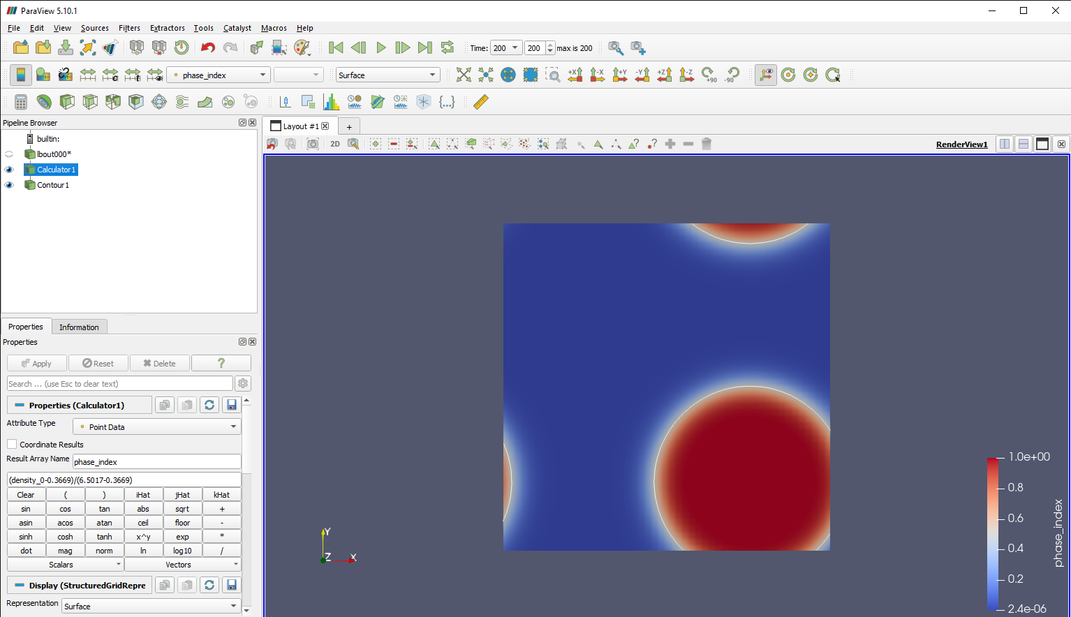
The Python script vtk_to_twophase.py can read the densities at all grid points in a VTK file, work out the minimum and maximum values as the vapour and liquid densities, and then calculate phase indices based on these values. It uses the phase indices to determine the centre of mass for the drop, which corresponds to the location of its centre, before finding a contour or isosurface as a series of interpolated points where \(\rho^N = 0.5\). A function for an ellipse or ellipsoid is then fitted to those points to work out the semi-axes for the drop, and the geometric mean of these is given as the drop radius.

To run this script, type the following command:

python vtk_to_twophase.py --vtkin lbout000200.vts

substituting lbout000200.vts with the name of the VTK file you wish to check, ideally one in which the system has equilibrated. If you wish to see the fit of the shape to the contour or isosurface, add --plot to the above command.

For the Shan-Chen calculation, the drop’s centre in the final snapshot is located at \((36.95, 10.31)\) and has a mean radius of \(R = 14.31 \Delta x\). For the free-energy calculation, the drop centre is located at \((22.79, 16.47)\) and has a mean radius of \(R = 14.52 \Delta x\).

Interfacial width and surface tension:

To determine the interfacial width, threshold values of the phase index \(\rho^N\) need to be selected at which the transition between bulk phases and the interface can be identified. Since the bulk liquid and vapour phases are likely to vary slightly in density from the maximum and minimum values respectively, the phase index threshold values cannot be 0 and 1 but should be a little way inside of these, i.e. \(\epsilon\) and \(1-\epsilon\). We recommend a value of \(\epsilon = 0.1\).

The Python script vtk_to_twophase.py can find the contours or isosurfaces where \(\rho^N = \epsilon\) and \(\rho^N = 1-\epsilon\), fit ellipses or ellipsoids to those shapes and determine the difference in radii between them as the interfacial width. Type the following command:

python vtk_to_twophase.py --vtkin lbout000200.vts --threshold 0.1

substituting 0.1 with the required value of \(\epsilon\). If you wish to include the interface plot, the two additional contours will be displayed only if the system is two-dimensional, as shown below for the Shan-Chen calculation.

For the Shan-Chen calculation, the interfacial thickness is estimated to be \(4.53 \Delta x\), while for the free-energy calculation it is estimated to be \(2.76 \Delta x\).

To determine the surface tension between the phases, we can exploit the Young-Laplace equation:

\[\Delta p = - \frac{2 \gamma}{R}\]

where the reciprocal of the drop radius is equal to the mean curvature at the interface. To obtain the pressure difference across the interface \(\Delta p\), we can use the vapour and liquid densities and the equation of state (including the parameters used for the calculation) to determine the pressures of both phases.

The same Python script can take the lbin.sys file used in the DL_MESO_LBE calculation as an additional input to specify the equation of state and its parameters, which can then be used to calculate the pressure difference and surface tension \(\gamma\). Type the following command:

python vtk_to_twophase.py --vtkin lbout000200.vts --lbin lbin.sys

substituting lbin.sys (if required) with the filename and location of the input file used for calculations.

For the Shan-Chen calculation, the surface tension is estimated to be \(\gamma \approx 0.06348\), while for the free-energy calculation it is \(\gamma \approx 0.040958\). The units for surface tension are equivalent to \(\rho_0 \frac{\Delta x^3}{\Delta t^2}\), where \(\rho_0\) is the equivalent ‘real-life’ density for \(\rho = 1\) in the LBE calculations.

It should be noted that the surface tension and the interfacial width for the free-energy calculation can be controlled using the specified surface tension parameter \(\kappa\), while these properties are generally not controllable for Shan-Chen calculations.

[Liu2010]

M Liu, Z Yu, T Wang, J Wang and LS Fan, A modified pseudopotential for a lattice Boltzmann simulation of bubbly flow, Chemical Engineering Science, 65, 5615-5623, 2010, doi: 10.1016/j.ces.2010.08.014.