Simulation Run
Step 1: It is important to rename the files output by DL_FIELD:
- Rename dl_poly.CONFIG to CONFIG
- Rename dl_poly.FIELD to FIELD
- Rename dl_poly.CONTROL to CONTROL
Step 2: Equilibration in DL_POLY
- Edit the CONTROL file, making the necessary changes (see CONTROL1). This CONTROL file instructs DL_POLY to run 200,000 MD steps at NVE ensemble, rescale the temperature to exactly 300K at every MD step. Using the variable timestep directive, enables DL_POLY to adjust the suitable timestep accordingly, especially at the early stage of simulation. This ensures the system dynamics are in control for high-energy conformations.
Title: Generic control file: CONTROL1
# This is a generic CONTROL file. Please adjust to your requirement.
# Directives which are commented are some useful options.

ensemble nve
temperature 300.0

# Perform zero temperature run (really set to 10K)
# zero

# Cap forces during equilibration, in unit kT/angstrom.
# (useful if your system is far from equilibrium)
#cap 1000.0

# Increase array size per domain
#densvar 10 %

# Bypass checking restrictions and reporting
#no index
#no strict
#no topolgy

steps 200000
equilibration steps 10000000
scale every 1
variable timestep 0.00001

cutoff 12.0
ewald precision 1e-6

# Need these for bond constrains
#mxshak 100
#shake 1.0e-6

# Continue MD simulation
restart

# traj 1 200 0
print every 1000
stats every 1000
job time 100000
close time 200
finish
Run the equilibration in DL_POLY:
$: ./dl_field
Repeat step 2 if necessary, by increasing the number of MD steps.
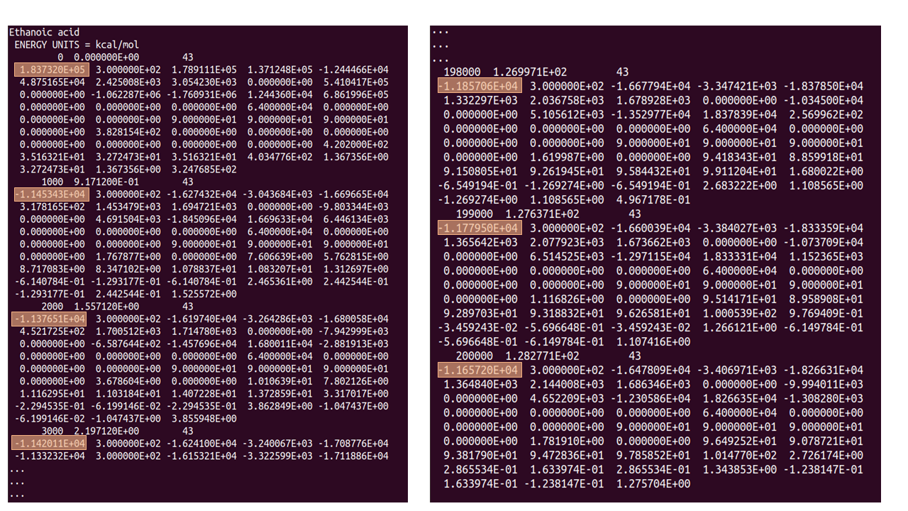
The figure above shows samples from the start (LHS) and end (RHS) of the STATIS file output from using the parameters as detailed in CONTROL1. The highlighted numbers show the total energy of the system -see how it fluctuates hugely at the beginning of the simulation and becomes more stable towards the end of the 200,000 steps.
Step 3: Checking your system is equilibrated
Check that the configurational energy values fluctuate around a mean value, when this has occurred equilibration has been reached. You can check this in the top entry of the LHS column of the STATIS file as shown above where the total energies are highlighted.
When you are satisfied a mean total energy value has been reached, reset the directive equilibration steps in the CONTROL file to zero. (See CONTROL2). Check if the energy values are steady without rescaling the temperature at approximately 300 K.
Title: Generic control file: CONTROL2
# This is a generic CONTROL file. Please adjust to your requirement.
# Directives which are commented are some useful options.

ensemble nve
temperature 300.0

# Perform zero temperature run (really set to 10K)
# zero

# Cap forces during equilibration, in unit kT/angstrom.
# (useful if your system is far from equilibrium)
#cap 1000.0

# Increase array size per domain
#densvar 10 %

# Bypass checking restrictions and reporting
#no index
#no strict
#no topolgy

steps 400000
equilibration steps 0
scale every 1
variable timestep 0.00001

cutoff 12.0
ewald precision 1e-6

# Need these for bond constrains
#mxshak 100
#shake 1.0e-6

# Continue MD simulation
restart

# traj 1 200 0
print every 1000
stats every 1000
job time 100000
close time 200
finish
Check if the energy values are steady without rescaling the temperature at approximately 300 K.
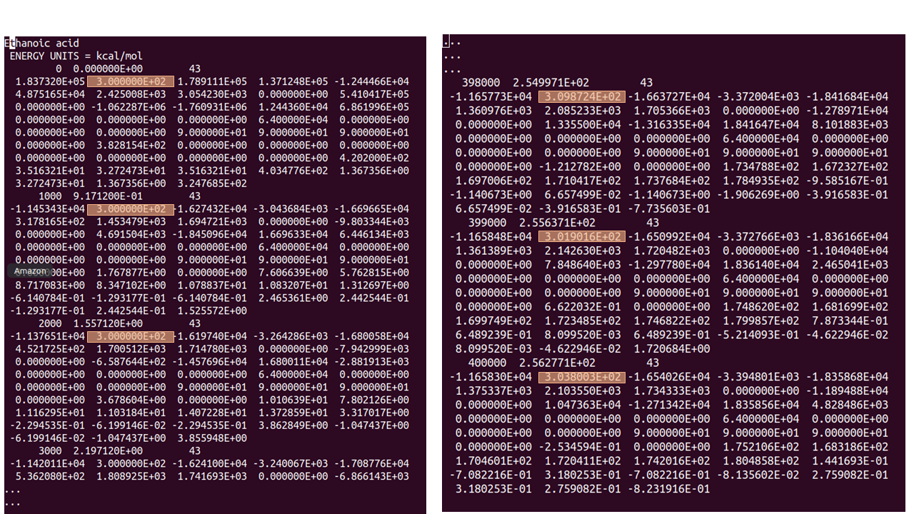
The figure above shows the temperature at the beginning of the re-run (LHS) - which for the first run was fixed at 300 K - and at the end (RHS), where the temperature decreases from ~310 K to ~304 K during the last three of the 400,000 MD steps. It is up to the user to decide if the temperature is sufficiently stable for their simulation.
Change to ensemble NPT to equilibrate the simulation box size (see CONTROL3), using restart noscale. If a further run is needed, restart the simulation and increase the MD steps in the CONTROL file.
Title: Generic control file: CONTROL3
# This is a generic CONTROL file. Please adjust to your requirement.
# Directives which are commented are some useful options.

ensemble npt hoover 0.4 1.0
temperature 300.0
pressure 0.00101325

# Perform zero temperature run (really set to 10K)
# zero

# Cap forces during equilibration, in unit kT/angstrom.
# (useful if your system is far from equilibrium)
#cap 1000.0

# Increase array size per domain
#densvar 10 %

# Bypass checking restrictions and reporting
#no index
#no strict
#no topolgy

steps 100000
equilibration steps 0
scale every 1
variable timestep 0.00001

cutoff 12.0
ewald precision 1e-6

# Need these for bond constrains
#mxshak 100
#shake 1.0e-6

# Continue MD simulation, from start
restart noscale

# traj 1 200 0
print every 1000
stats every 1000
job time 100000
close time 200
finish
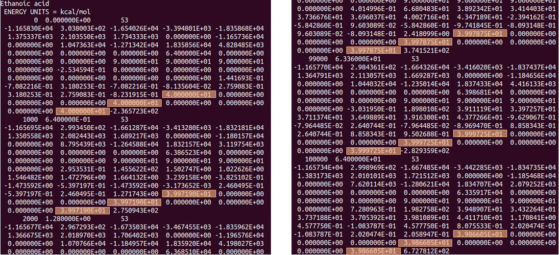
The figure above shows the simulation box lengths x, y, z (highlighted) at the beginning of the simulation (LHS) and at the end (RHS). After 100,000 steps of MD simulation the cell lengths remain at ~ 40 angstrom
Warning
Remember to run the copy script (e.g. copy.sh in the Resources/Molecular Simulations- Tools section) after each MD run, before carrying on for the next run. THEN edit the CONTROL file to increase the number of timesteps (which is cumulative).
Note
Changing the timestep value, or changing from variable to fixed timestep, or changing the ensemble necessitates using the restart noscale directive in the CONTROL for the first run. This instructs DL_POLY to restart a fresh MD run, which starts at 0 MD time and where the initial velocities of the system are derived from the CONFIG file. After that, ‘noscale’ needs to be removed if you want to run more MD steps. The directive noscale instructs DL_POLY to start a fresh simulation where the MD time starts from zero, and the initial velocity information is taken from the CONFIG file, rather than generated randomly.
Step 4: Sampling Run in DL_POLY (CONTROL4)
- Using the final CONFIG file from step 3, do the sampling run by producing the HISTORY trajectory files (see CONTROL4). Again, the directive restart noscale is used, to ensure the MD time starts from zero as the HISTORY file is produced. A fixed timestep of 0.0005 ps (0.5 fs) is also used.The directive traj 1 200 0 means the system configuration will be written out every 200 MD steps and contains only the positions of the atoms (this excludes velocities and forces).
Title: Generic control file: CONTROL4
# This is a generic CONTROL file. Please adjust to your requirement.
# Directives which are commented are some useful options.

ensemble npt hoover 0.4 1.0
temperature 300.0
pressure 0.00101325

# Perform zero temperature run (really set to 10K)
# zero

# Cap forces during equilibration, in unit kT/angstrom.
# (useful if your system is far from equilibrium)
#cap 1000.0

# Increase array size per domain
#densvar 10 %

# Bypass checking restrictions and reporting
#no index
#no strict
#no topolgy

steps 100000
equilibration steps 0
scale every 1
timestep 0.0005

cutoff 12.0
ewald precision 1e-6

# Need these for bond constrains
#mxshak 100
#shake 1.0e-6

# Continue MD simulation, from start
restart noscale

traj 1 200 0
print every 10000
stats every 10000
job time 1000000
close time 200
finish
After the first sampling run, remember to remove the ‘noscale’ directive in the CONTROL before doing a further run. For each successive run, the trajectory will append onto the existing HISTORY file.
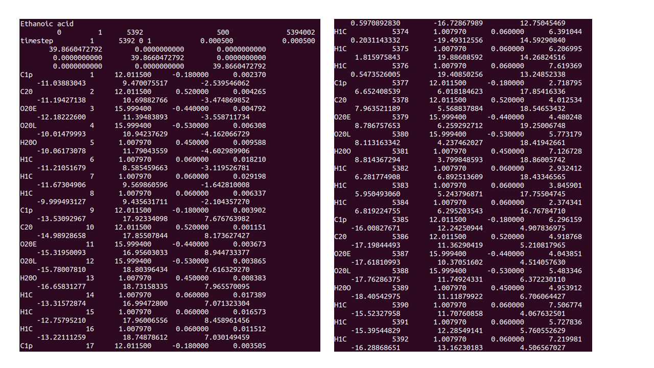
The figure above shows the HISTORY output at the beginning (LHS) and end (RHS) of the first sampling run of 100,000 MD steps. It’s up to the user to decide the length of the required simulation sampling run.
| TIP: | Rather than producing one large HISTORY file, after each run, the HISTORY file can be renamed serially (for instance HISTORY1, HISTORY2, etc). In this way, the next simulation run will produce a new HISTORY file. |
|---|
Finally, when you are satisfied the simulation sampling run is complete, copy the REVCON file to CONFIG (or use the latest HISTORY file) and view it in VMD e.g.
$: cp REVCON CONFIG
$: vmd &
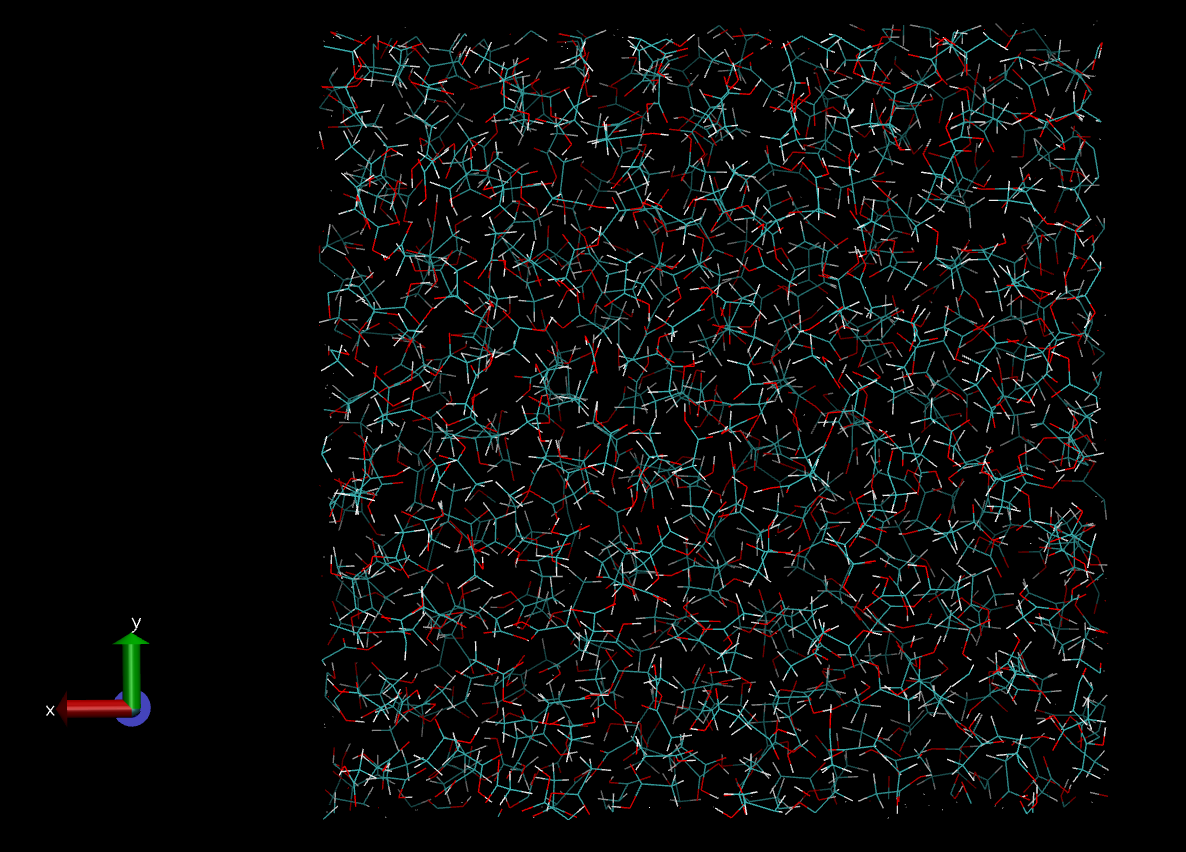
Note how there is a complete lack of order in the output configuration (contrast this with the output from DL_FIELD in the Section Sample Preparation.