Using DL_MESO_LBE¶

Summary¶

DL_MESO_LBE uses a number of input files to read in the details of an LBE simulation and produces output files containing the results. The Java GUI and utilities supplied with DL_MESO can be used to create/modify LBE simulation inputs and work with outputs to enable users to visualise and analyse simulations.

Input files¶

Two input files are required for a DL_MESO_LBE calculation:

lbin.sys: gives simulation controls, specifying properties such as lattice scheme, grid size, number of timesteps, relaxation times, properties for initial and boundary conditions etc.
lbin.spa: provides information on which lattice sites include boundary conditions and their types.

DL_MESO_LBE will ordinarily set up the initial state of the LBE calculation (fluid velocities, densities etc.) using the initial conditions specified in lbin.sys for every grid point. It is possible, however, to supply your own using an lbin.init file to specify fluid velocities, densities etc. at any grid point that should not use the defaults. The easiest way to create an lbin.init file is to use one of the utilities (see below) to either specify the locations, sizes and content of drops or to process the restart file (lbout.dump) generated by a previous DL_MESO_LBE calculation.

These files are in text format and can be opened, created or modified by hand using your favourite text editor. However, the format for lbin.spa files can be difficult to read and understand: I would therefore recommend using the GUI supplied with DL_MESO to create these files.

lbin.sys¶

An edited extract from a lbin.sys file used in LBE Exercise 2 is shown here.

space_dimension              2
discrete_speed               9
number_of_fluid              2
number_of_solute             0
temperature_scalar           0
phase_field                  0
grid_number_x                150
grid_number_y                50
grid_number_z                1
domain_boundary_width        1
incompressible_fluids        0
collision_type               BGKGuo
interaction_type             Lishchuk
output_format                VTK
output_type                  Binary
total_step                   400000
equilibration_step           5000
save_span                    500
relaxation_fluid_0           1.0
relaxation_fluid_1           1.0
density_ini_0                2.0
density_ini_1                0.0
density_inc_0                2.0
density_inc_1                2.0
speed_top_0                  0.005
speed_top_1                  0.0
speed_top_2                  0.0

Each line consists of keywords separated by underscores to indicate a property and either a number or a word to specify the value for that property. The first ten lines shown here - specifying the numbers of dimensions, discrete speeds, fluids, solutes, temperature scalar, phase field, grid points in \(x\)-, \(y\)- and \(z\)-directions and the domain boundary width - are compulsory for all simulations, although the lines do not have to be in any particular order.

The lattice scheme is defined by the numbers of dimensions and discrete speeds: the four lattices currently available in DL_MESO_LBE are D2Q9, D3Q15, D3Q19 and D3Q27, where \(\textrm{D}n\textrm{Q}m\) denotes \(n\) dimensions and \(m\) lattice links per grid point. The keywords domain_boundary_width indicates how many lattice points are needed as a boundary halo for parallel calculations [1]. The keywords collision_type indicate both the collision scheme and how forces (externally applied and those arising from fluid interfaces) are included, while interaction_type is used to select the mesoscopic interaction scheme.

The relaxation times (\(\tau\)) for each fluid (numbering starting from 0) are given with relaxation_fluid_* keywords. The initial density for each fluid throughout the system is given by density_ini_*, while constant densities used for incompressible fluids and some mesoscopic interactions are given by density_inc_* [2].

Properties for boundary conditions applying e.g. constant densities or velocities can be specified. In this case, speed_top_* indicates the velocity of all fluids at the top boundary of the box (with 0, 1 and 2 indicating \(x\)-, \(y\)- and \(z\)-components respectively). These boundary conditions do not apply during any equilibration timesteps specified by equilibration_step.

There are a few options available for the output_format - snapshots of the simulation showing fluid velocities, densities etc. at all grid points - which are written every save_span timesteps either from the start or after equilibration.

Further details of available keywords in this file can be found in Chapter 6 of The DL_MESO User Manual.

lbin.spa¶

A short extract from a lbin.spa file used in LBE Exercise 2 is shown here.

The format consists of lines with grid point coordinates followed by a code for the required boundary condition at that point. A full list of the available boundary condition codes can be found in Chapter 6 of the The DL_MESO User Manual, but it is much easier to create an lbin.spa file using the GUI (see below).

Output files¶

The outputs from DL_MESO_LBE can include:

Screen/standard output: summary of the LBE simulation with ongoing timings, fluid masses and system momenta.
lbout.dump: state of simulation recorded at time intervals, continuously overwritten (last one provided) - written in binary, can be used to restart simulation or used with utilities.
lbout*.vts: simulation trajectory as snapshots at user-specified time intervals - written in structured grid XML-based VTK format for opening in Paraview, includes macroscopic velocity, fluid densities etc. at each grid point.

By default, the MPI parallel version of DL_MESO_LBE will write an output file per outputting timestep for each processor core. This number can be reduced by using the keywords output_combine_x etc. in lbin.sys to gather data among cores in each direction before writing: selecting this option for all three dimensions will produce a single output file per timestep.

Further details of these file formats can be found in Chapter 6 of The DL_MESO User Manual.

Running DL_MESO_LBE¶

Before running DL_MESO_LBE, first ensure your working directory (dl_meso/LBE) includes at least lbin.sys and lbin.spa files.

To launch DL_MESO_LBE to run on a single processor, type in the following command:

./lbe.exe

This will work for both serial and parallel versions of the code, with or without OpenMP multithreading. To run an MPI-parallelised version of DL_MESO_LBE on more than one processor core, you have to use a command - either mpirun or mpiexec, depending on your MPI installation - that uses MPI runtime libraries and specifies how many processor cores to use. For example, to launch DL_MESO_DPD on 4 processor cores, type:

mpirun -np 4 ./dpd.exe

By default, you will see messages appear on the screen as DL_MESO_LBE runs to show how the calculation is progressing. You can redirect this to a file (e.g. output.txt) for future reference by adding one of the following to the end of your launch command:

> output.txt
| tee output.txt

where the first will write the standard output to the file without displaying it on the screen, while the second will write the output to the file and display it on the screen.

Running GUI¶

Some of the tasks in the practical LBE exercises can make use of the GUI. You can launch it from dl_meso/WORK with the command:

java -jar ../JAVA/GUI.jar

A runscript in this directory (rungui) can alternatively be used to launch the GUI. When the GUI launches, click on the LBE button at the top. A sidebar on the left hand side will appear with more buttons for LBE simulations.

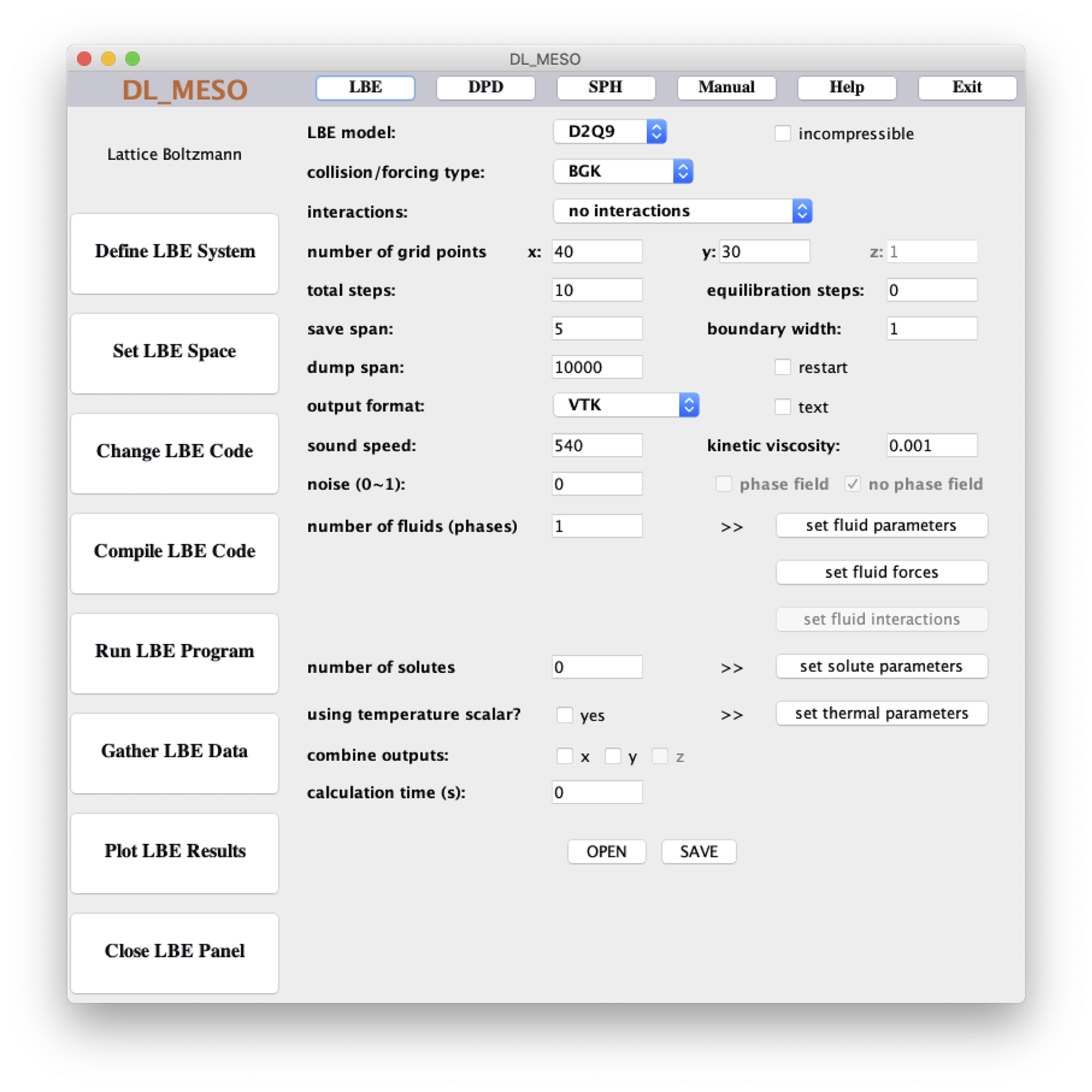
Define LBE System section of GUI to create and edit lbin.sys files for DL_MESO_LBE

The first button, Define LBE System, brings up some pulldown boxes and text fields to help you create a new lbin.sys file or edit a pre-existing one in the directory where you launched the GUI. If you wish to open the lbin.sys in your working directory, click OPEN to load it into the GUI.

Clicking on the active buttons will open pop-up windows with further fields to specify e.g. fluid parameters, fluid interactions: any values you enter will only be included in the lbin.sys file if you click the SAVE button for that window. Once you have completed entering values for your simulation, clicking on SAVE in the main window will create a new lbin.sys file with those values and overwrite any existing file.

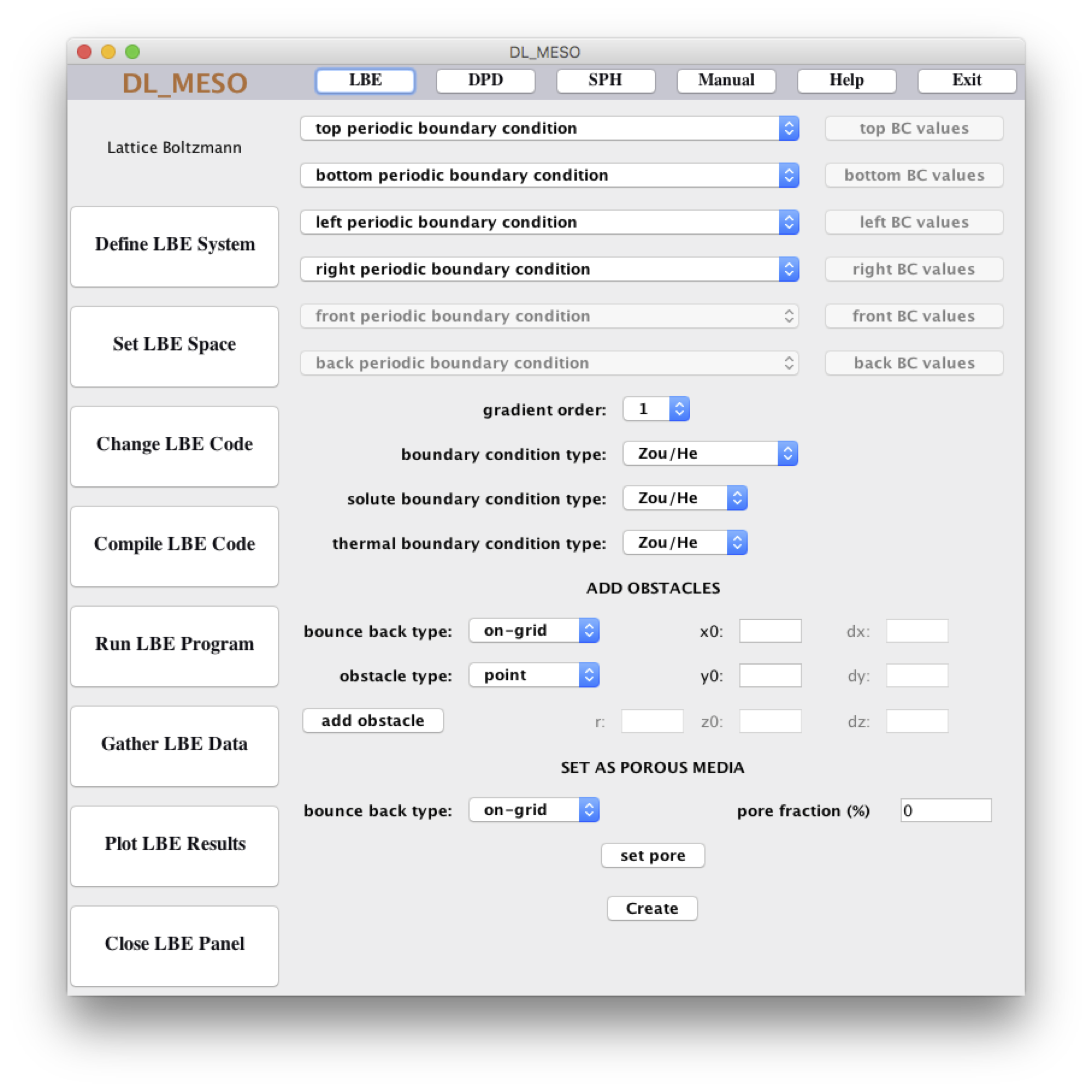
Set LBE Space section of GUI to create lbin.spa files for DL_MESO_LBE

The second button, Set LBE Space, brings up some more pulldown boxes, buttons and text fields to specify boundary conditions for your LBE simulation. This section can only be used once you have opened or saved an lbin.sys file in the Define LBE System window and cannot open an existing lbin.spa file.

The pulldown boxes at the top of the window can be used to specify boundary conditions at the edges of the simulation box. If any of the selected conditions require values for velocities, fluid densities etc., the button next to the pulldown box will become active and clicking it will open a pop-up window where you can specify the required values. (You must click SET BC to store the values in memory.)

You can add obstacles with bounce-back boundaries - individual points, spheres, cylinders/circles or rectangular/cuboidal blocks - in the ADD OBSTACLES section. To add an obstacle, select the type in the pulldown box, enter the details - position at its centre or bottom left corner, radius or extent - and click add obstacle. The SET AS POROUS MEDIA section allows you to create randomised porous media for your simulations by selecting the type of bounce-back condition, entering the pore fraction (in percent) and clicking set pore. Note that neither of these options displays anything on screen when you click the buttons, but they will take effect when the lbin.spa file is created.

Once you have finished specifying boundary conditions, clicking Create will create a new lbin.spa file with the boundary conditions and append any boundary values to lbin.sys.

Further details on what the GUI can do and how to use it can be found in Chapter 3 of The DL_MESO User Manual.

DL_MESO_LBE utilities¶

One LBE utility will help you set up a simulation, some LBE utilities will process output files (*.vts) to make them easier to visualise in Paraview, some will read the lbout.dump file and produce more useable outputs. The executables for the most useful utilities are:

init.exe: creates a lbin.init file to specify initial velocities, densities etc. different to those specified in lbin.sys - can be used to insert circular/spherical fluid drops;
vtk.exe: gathers together data in XML-based VTK files after running DL_MESO_LBE in parallel by creating linking files (lbout*.pvts) to put together *.vts files from individual processor cores when plotting in Paraview;
dump_to_init.exe: creates a lbin.init file from a previous simulation’s lbout.dump restart file.

These can be launched in the working directory in a similar fashion to running DL_MESO_LBE on a single processor core, e.g.

./init.exe

although some utilities can take command-line options to change how they work. (The utility init.exe will prompt the user to enter information.) Every utility can take -h as an option to show what the utility does and what the other available options happen to be.

Footnotes

[1]	When running DL_MESO_LBE in serial, no boundary halo is required as any periodic boundaries are implemented using modulo functions on grid positions. This value should still be specified in case the simulation is run in parallel later, but it will be ignored for serial runs.

[2]	One of the utilities (init.exe) uses the constant densities as defaults when setting up initial conditions, e.g. when including immiscible drops in the calculation.