Using DL_MESO_DPD

Summary

DL_MESO_DPD uses a number of input files to read in the details of a DPD simulation and produces output files containing the results. The Java GUI and utilities supplied with DL_MESO can be used to create/modify DPD simulation inputs and work with outputs to enable users to visualise and analyse simulations. Three Python3 scripts are also supplied for this workshop to make it easier to carry out a simulation workflow for one of the DPD exercises and to examine the contents of an output file produced by DL_MESO_DPD.

Input files

Two input files are required for a DL_MESO_DPD calculation:

• CONTROL: gives simulation controls, specifies properties such as timestep size, temperature, number of timesteps, ensemble type etc.
• FIELD: provides definitions and numbers of beads, specifies interactions between them, the contents and connectivity of any molecules and any external fields.

DL_MESO_DPD will ordinarily devise an initial configuration (positions, velocities and forces for particles) based on the contents of the FIELD file. It is possible, however, to supply your own using a CONFIG file to specify particle positions etc. The easiest way to create a CONFIG file is to use one of the utilities (see below) to process the restart file (export) generated by a previous DL_MESO_DPD calculation.

These files are in text format and can be opened, created or modified by hand using your favourite text editor. (CONTROL and FIELD files also be created or modified using DL_MESO’s GUI.) If you have previously used DL_POLY for molecular dynamics calculations, you may notice many similarities in the names, formats and content of these files.

CONTROL

An example of a CONTROL file used in DPD Exercise 2 is shown here.

DL_MESO lipid bilayer example

volume 16384.0
temperature 1.0
cutoff 1.0
boundary halo 2.0

timestep 0.03
steps 100000
equilibration steps 0
scale temperature every 100
trajectory 0 2000
stats every 2000
stack size 100
print every 1000
job time 10800.0
close time 100.0

ensemble nvt mdvv

finish

The first line gives a title for the simulation for your own reference. Subsequent lines use keywords to specify properties required for the simulation, - volume, temperature etc. - which are normally followed by the required value or values in the same line, all separated by spaces, commas or tabs. Many of these are clearly understandable and are explained fully in Chapter 10 of The DL_MESO User Manual, although the following are worth noting here:

• volume specifies the volume of the simulation box. If a single number follows this keyword, the box is assumed to be cubic, while using three numbers specifies the box sizes for each dimension.
• boundary halo specifies how far to search into the neighbouring section of the box for particles to ensure all interaction forces are calculated correctly. This needs to be at least as large as the maximum interaction cutoff, but may need to be larger if bond interactions are included.
• trajectory specifies at which number timestep trajectory data should be written to a HISTORY file, how often that data should be written and (optionally) which data should be written (0 or no value = positions, 1 = positions and velocities, 2 = positions, velocities and forces).
• stats specifies how often calculated properties for the system (potential energy, pressure, stress tensor, temperature etc.) should be written to a CORREL file.
• stack size specifies how many timesteps of calculated properties should be stored to calculate rolling averages shown in the OUTPUT file.
• print specifies how often (in timesteps) a summary of the simulation should be written to the OUTPUT file.
• job time and close time are mainly for running on supercomputers that require batch scripts to submit jobs, indicating how long the simulation should run for and the time DL_MESO_DPD needs to write data to files for a later restart (both in seconds).
• ensemble nvt mdvv indicates the ensemble used for the simulation - constant volume and temperature (NVT) - and how the DPD thermostat should be applied (using Velocity Verlet integration as usually applied in MD).

The last line read by DL_MESO_DPD contains the keyword finish.

FIELD

An example of a FIELD file used in DPD Exercise 2 is shown here.

DL_MESO lipid bilayer example

SPECIES 3
H        1.0 0.0 0
C        1.0 0.0 0
W        1.0 0.0 35152

MOLECULES 1
HC6
nummols 2000
beads 7
H        -0.0172847 0.383451 0.2849
C        -0.016165 0.381111 -0.215093
C        0.280007 0.0703806 0.0412832
C        0.440339 -0.359403 -0.157664
C        0.00469362 -0.136529 -0.260333
C        -0.455453 -0.119133 -0.0654933
C        -0.236136 -0.219878 0.3724
bonds 6
harm  1 2 128.000 0.500000
harm  2 3 128.000 0.500000
harm  3 4 128.000 0.500000
harm  4 5 128.000 0.500000
harm  5 6 128.000 0.500000
harm  6 7 128.000 0.500000
angles 5
cos   1 2 3 20.0 0.0 1.0
cos   2 3 4 20.0 0.0 1.0
cos   3 4 5 20.0 0.0 1.0
cos   4 5 6 20.0 0.0 1.0
cos   5 6 7 20.0 0.0 1.0
finish

INTERACTIONS 6
H H dpd 25.0 1.0 4.5
C C dpd 25.0 1.0 4.5
W W dpd 25.0 1.0 4.5
H W dpd 35.0 1.0 4.5
H C dpd 50.0 1.0 9.0
C W dpd 75.0 1.0 20.0

close

The first line gives a title for the simulation for your own reference. This is followed by a number of sections starting with a keyword - SPECIES, INTERACTIONS, MOLECULES - that specify the numbers of particle species, pairwise interactions and molecule types respectively.

The SPECIES keyword is followed by lines defining each particle species, giving the name, mass, charge, the number of particles for the species not included in molecules - usually indicating which species is the solvent - and (optionally) whether or not the particles are frozen in place (1 if they are, 0 or no value if they are not).

The INTERACTIONS keyword is followed by lines indicating which two particle species are involved in an interaction, the functional form (dpd in this case referring to ‘standard’ Groot-Warren), the conservative force parameter \(A_{ij}\), the cutoff distance \(r_{c,ij}\) and the dissipative force parameter \(\gamma_{ij}\). Not all species pairs necessarily have to have interactions specified, as mixing rules can be used to fill in missing information.

The MOLECULES keyword is followed by definitions for each molecule type. These start with the name of the molecule type, followed by further keywords for the number of molecules in the simulation (nummols), the number of beads per molecule, the numbers of bonds, angles and dihedrals per molecule [1], and finish to indicate the end of the definition for that molecule. Under beads, lines follow to indicate the species of each bead in the molecule and sample coordinates used to insert the molecule in the box when creating an initial system configuration (i.e. when no CONFIG file is supplied). The keywords bonds, angles and dihedrals are followed by lines showing the type of bond/angle/dihedral interaction, the pair/triple/quadruple of particles in each molecule involved (referring to the list of beads) and the parameters for the bond/angle/dihedral interaction. (Details of these can be found in Chapter 10 of The DL_MESO User Manual.)

The keyword close indicates to DL_MESO_DPD that the end of the FIELD file has been reached.

Output files

The output files from DL_MESO_DPD can include:

• OUTPUT: gives a summary of the DPD simulation, including input information, timing, statistical properties (e.g. energies, pressure, temperature) at given timesteps and averages over the simulation.
• CORREL: gives tabulated instantaneous values of calculated properties at user-specified time intervals, which can be read and plotted using e.g. Excel, gnuplot.
• HISTORY: trajectory data (i.e. simulation snapshots at user-specified time intervals) - written in binary, requires utilities to read and use.
• export: state of simulation recorded at time intervals, continuously overwritten (last one provided) - written in binary, can be used to restart simulation or used with utilities.
• REVIVE: statistical accumulators and random number generator states for simulation, continuously overwritten - written in binary, can be used to restart simulation.

The output file formats for DL_MESO_DPD (HISTORY, export and CORREL) are deliberately agnostic, in the sense that they are not designed to be read by a single proprietary program. The utilities supplied with DL_MESO (see below) can convert this data into specific formats, but if you are able to write your own programs or scripts, you can get the data into the format of your choice.

Further details of these file formats can be found in Chapter 10 of The DL_MESO User Manual and in Chapter 11 of The DL_MESO Technical Manual.

Running DL_MESO_DPD

Before running DL_MESO_DPD, first ensure your working directory (dl_meso/WORK) includes at least CONTROL and FIELD files.

To launch DL_MESO_DPD to run on a single processor, type in the following command:

./dpd.exe

This will work for both serial and parallel versions of the code, with or without OpenMP multithreading. To run an MPI-parallelised version of DL_MESO_DPD on more than one processor core, you have to use a command - either mpirun or mpiexec, depending on your MPI installation - that uses MPI runtime libraries and specifies how many processor cores to use. For example, to launch DL_MESO_DPD on 4 processor cores, type:

mpirun -np 4 ./dpd.exe

By default, no messages will be displayed on screen while DL_MESO_DPD runs. You can either add the directive l_scr to the CONTROL file to redirect what normally gets written to OUTPUT to the screen, or open a new terminal window or tab in the working directory and type:

tail -f OUTPUT

to see what gets written to OUTPUT continuously as DL_MESO_DPD runs.

Running GUI

There is no real need to use the GUI for these practical DPD exercises, but you can launch it from dl_meso/WORK with the command:

java -jar ../JAVA/GUI.jar

A runscript in this directory (rungui) launches the GUI using the same command while being easier to remember. Details on what the GUI can do and how to use it can be found in Chapter 3 of The DL_MESO User Manual.

DL_MESO_DPD utilities

Most of the DPD utilities will read the HISTORY or export files and produce more useable outputs. The executables for the most useful ones are:

• traject_vtf.exe: reads the HISTORY file’s trajectories and writes a trajectory file (traject.vtf) that can be read and visualised by VMD;
• traject_xml.exe: reads the HISTORY file’s trajectories and writes a series of trajectory files (traject_*.xml) that can be read and visualised by OVITO;
• local.exe: calculates instantaneous and time-averaged localised properties (densities, velocities, stress tensors) from HISTORY file trajectories by summing properties in user-specified slices of the system (in a similar fashion to histograms), can be visualised and analysed using Paraview;
• isosurfaces.exe: calculates isosurfaces of a specified particle species (that can be visualised in Paraview) and an order parameter to determine mesophases;
• rdf.exe: calculates radial distribution functions (RDFs) from HISTORY file trajectories;
• export_config.exe: converts the simulation snapshot in export files into a CONFIG file (to allow new simulations starting from that configuration);
• molecule.exe: determines inputs required to include molecules in DPD simulations, including sample configurations, bond connectivity etc. and writes them to the FIELD file.

These can be launched in the working directory in a similar fashion to running DL_MESO_DPD on a single processor core, e.g.

./traject_vtf.exe

although each utility can take command-line options to change how they work. Every utility can take -h as an option to show what the utility does and what the other available options happen to be.

Python scripts

To help with the DPD exercises, I have provided three Python3 scripts for you to use. These can help you automate simulation workflows, visualise and analyse the results of DL_MESO_DPD simulations: they are not absolutely essential and you can still carry out the exercises without them, but they will speed things up!

If you would like to make use of these scripts, I suggest putting a copy of each one into your working directory with the various executables for DL_MESO_DPD.

flory_huggins.py

flory_huggins.py is a simulation workflow script to carry out a series of DL_MESO_DPD simulations of two separating species. These simulations are designed to obtain a relationship between DPD conservative force parameters \(A_{ij}\) and the Flory-Huggins \(\chi\)-parameters (see DPD Exercise 1: DPD, hydrophobicity and parameterisation for more details).

It creates the required input files - CONTROL, CONFIG and FIELD - to carry out these simulations for various values of \(A_{ij}^{\text{AB}}\), launches the simulations one-by-one, obtains a time-averaged local concentration profile for one bead species and adds these profiles to a text file for later analysis. It also calculates a value of \(\chi\) for each simulation and estimates its error.

To use the script, invoke it with your Python3 interpreter with one of the following commands (the latter if permissions on the script allow it to be executed):

python flory_huggins.py
python3 flory_huggins.py
./flory_huggins.py

You can add a number of optional command-line options at the end of the invocation:

• --rho <rho> sets the overall particle density of the simulations to <rho> (equal to 3 by default)
• --Aii <Aii> sets the conservative force parameter between beads of the same species (\(A_{ij}^{\text{AA}} = A_{ij}^{\text{BB}}\)) to <Aii> (equal to 25.0 by default)
• --Aijmin <Aijmin> sets the minimum conservative force parameter between beads of the two different species (\(A_{ij}^{\text{AB}}\)) to <Aijmin> (equal to 33.0 by default)
• --Aijmax <Aijmax> sets the maximum conservative force parameter between beads of the two different species (\(A_{ij}^{\text{AB}}\)) to <Aijmax> (equal to 43.0 by default)
• --dA <dA> sets the interval of unlike species conservative force parameter between simulations to <dA> (equal to 1.0 by default)
• --dx <dx> sets the spacing of histogram bins for concentration profiles to <dx> (equal to 0.1 by default)
• --L <L> sets the length of the box along the x-direction to <L> (equal to 20.0 by default)
• --W <W> sets the width of the box in the y- and z-directions to <W> (equal to 8.0 by default)
• --print-to-screen will redirect the summary of each simulation to the screen instead of writing to an OUTPUT file
• --nproc <nproc> sets the number of processor cores to run DL_MESO_DPD (defaults to 1 core, i.e. serial running)

The results - the \(\chi\) value and its standard deviation, followed by the concentration profile for each simulation - will be placed in a file called floryhuggins-rho-<rho>.dat, which is designed to be read by flory_huggins_plot.py. Subsequent runs of flory_huggins.py for the same density will append data to this file if it already exists.

flory_huggins_plot.py

flory_huggins_plot.py will visualise the results from flory_huggins.py using the generated text file. You can look at the local concentration profiles generated from the DL_MESO_DPD simulations, recalculate \(\chi\) values for each set of conservative force parameters, plot these values and find a relationship between \(\chi^{\text{AB}}\) and \(A_{ij}^{\text{AB}} - A_{ij}^{\text{AA}}\).

To use the script, invoke it with your Python3 interpreter using one of the following commands:

python flory_huggins_plot.py
python3 flory_huggins_plot.py
./flory_huggins_plot.py

You can optionally add the command-line option --rho <rho>, which chooses data for the system-wide particle density <rho> (which is equal to 3.0 by default).

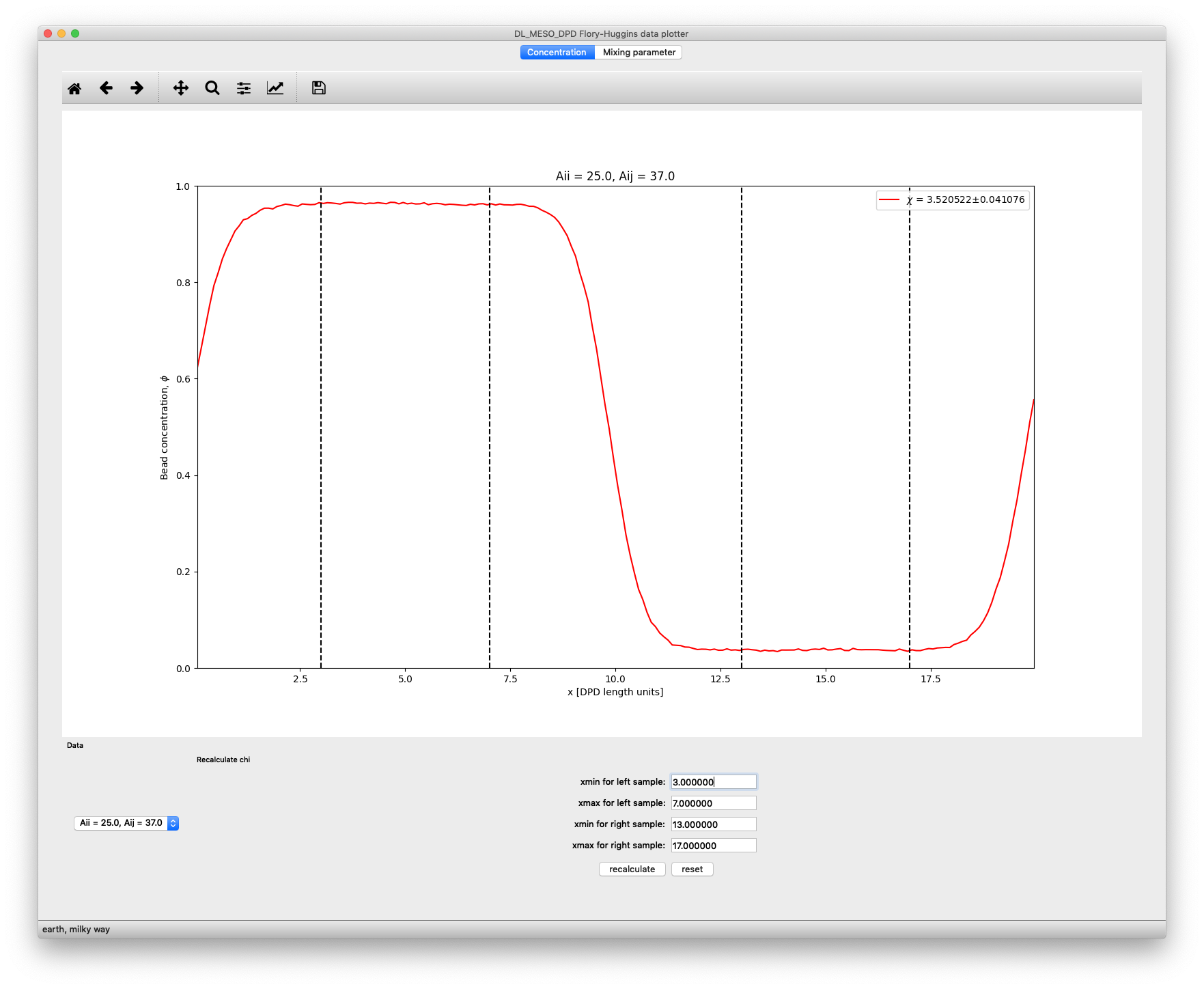
Plot of concentration profile shown in flory_huggins_plot.py

The Concentration tab allows you to plot the local concentration profile for each simulation: a pulldown box at the bottom left of the window will allow you to choose the simulation. The legend box includes the value of \(\chi^{AB}\) obtained for this simulation, along with an estimate of the standard deviation of this value.

If you want to modify this value, you can choose to recalculate it by choosing the extents used to sample higher and lower concentrations. The positions of these lines can be changed using the text boxes at the bottom of the window, and the recalculate button can be used to obtain a new value (and standard deviation) for \(\chi^{\text{AB}}\). The reset button can be used to go back to the original values of \(\chi^{\text{AB}}\) as provided with the concentration data.

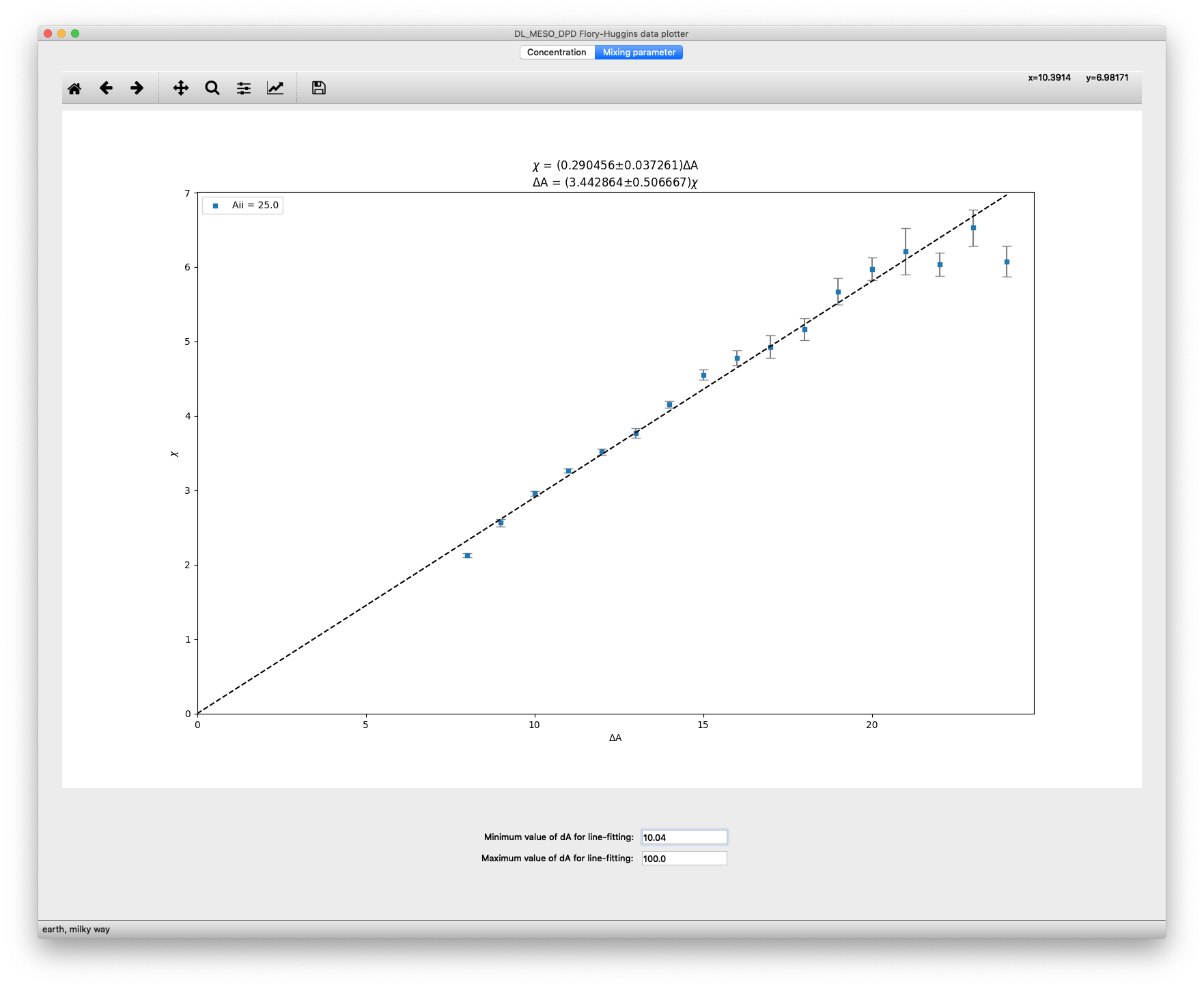
Plot of \(\chi^{\text{AB}}\) as a function of \(\Delta A_{ij}\) shown in flory_huggins_plot.py

The Mixing parameter tab gives a plot of \(\chi^{\text{AB}}\) as a function of \(\Delta A_{ij} = A_{ij}^{\text{AB}} - A_{ij}^{\text{AA}}\). If you have used multiple values of the like-like conservative force parameter \(A_{ij}^{\text{AA}}\), data for different values of this parameter will be plotted in different colours (as indicated by the legend box in the top left). The standard deviations for each data point are indicated using error bars.

Assuming the relationship between \(\chi^{\text{AB}}\) and \(\Delta A_{ij}\) to be entirely proportional, a dashed line indicating the best fit of available data to a linear plot with zero at the origin is included. The equations for this best-fit line are given at the top of the plot with errors indicating the extremes of the gradient.

Since data below and above certain values of \(\Delta A_{ij}\) may not be reliable, you can change the minimum and maximum values of this property used to calculate the best-fit line in the text boxes at the bottom of the window.

dlmresultviewer.py

dlmresultviewer.py is a more general-purpose script to plot and analyse the results from DL_MESO_DPD, using any of the following files if available:

• CORREL with calculated properties for the system
• RDFDAT with radial distribution functions
• MSDDAT with mean-squared displacements
• A VTK file ending with .vtk or .vts containing local values of properties calculated for voxels (volume divisions)

To use the script, invoke it with your Python3 interpreter with one of the following commands:

python dlmresultviewer.py
python3 dlmresultviewer.py
./dlmresultviewer.py

You can add up to two optional command-line options at the end of the invocation:

• --cor <correl> sets the name of the CORREL file to <correl> (default: CORREL)
• --rdf <rdfdat> sets the name of the RDFDAT file to <rdfdat> (default: RDFDAT)
• --msd <msddat> sets the name of the MSDDAT file to <msddat> (default: MSDDAT)
• --loc <local> sets the name of the VTK file with localised properties to <local> (default: averages.vtk)

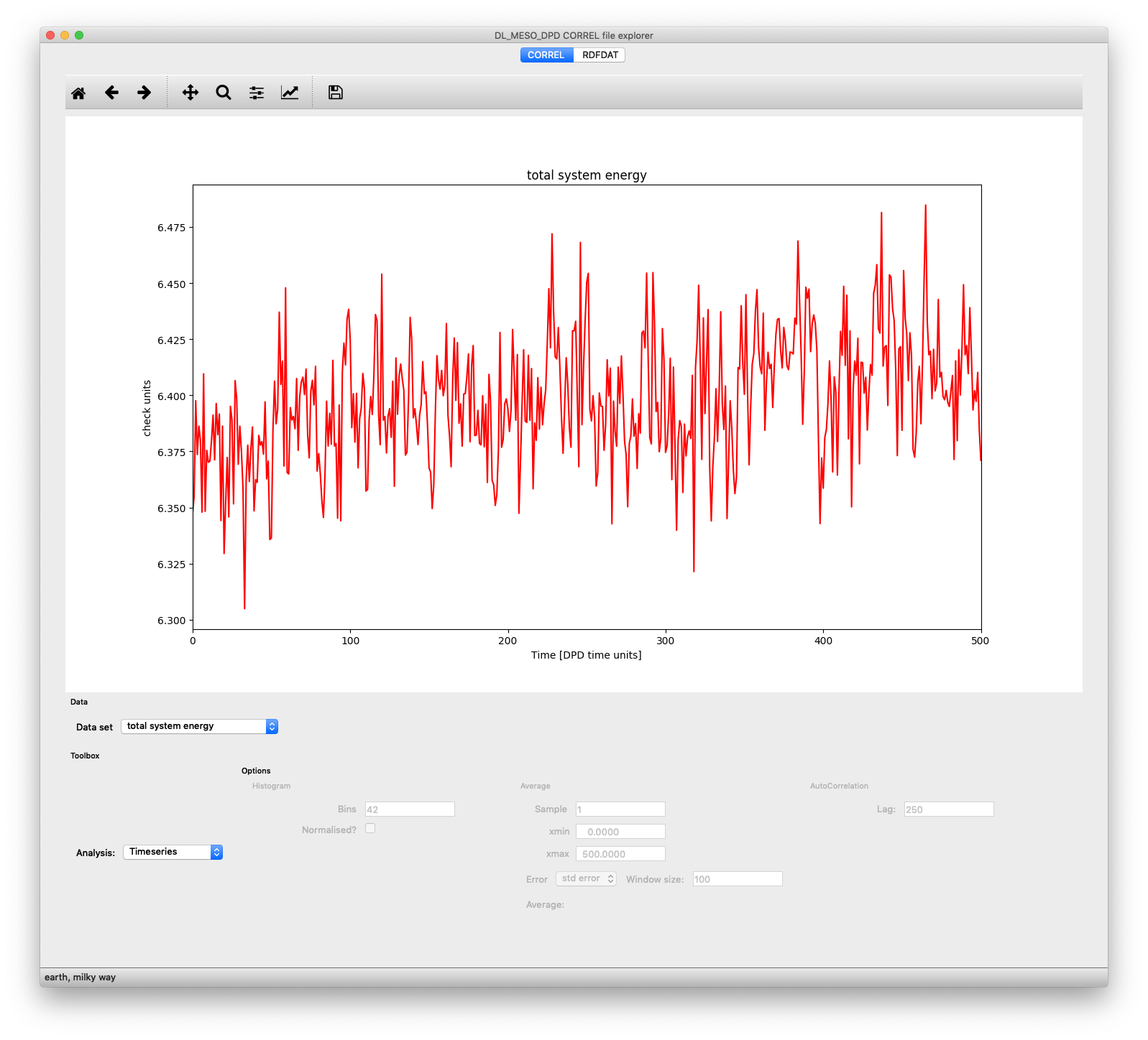
Plot of total system energy per particle as a function of time, obtained from a CORREL file, shown in dlmresultviewer.py

When the script is launched, it looks for any of the four kinds of file and, if it finds any, opens the main window and creates tabs for each file, where its data can be plotted and analysed. For a CORREL file, there are two pulldown boxes at the bottom left of the window: Data set selects which system property you wish to visualise - the list of which depends on the contents of the CORREL file - while Analysis selects what you want to do with the selected data. You can plot one of the following for a given property:

• A simple Timeseries
• A Histogram of the values obtained during the simulation
• A time series with a Running average added (also providing a measure of mean and standard error)
• An Autocorrelation with respect to time
• A Fourier transform

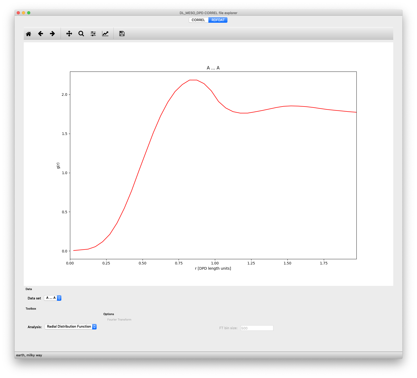
Plot of radial distribution function between particle species pair A-A, obtained from an RDFDAT file, shown in correl.py

If an RDFDAT file is available after running the rdf.exe utility or an equivalent Python script, the tab for this file will be populated with a plotting window. The Data set pulldown box allows you to select which pair of particle species you wish to plot, while the Analysis pulldown box allows you to choose to plot the raw Radial Distribution Function or its Fourier Transform (related to the structure factor). The plot for the latter can also depend upon the number of bins used to calculate the Fourier transform, which can be modified using the text box at the bottom of the window.

If an MSDDAT file is available after running the msd.exe utility or an equivalent Python script, the tab for this file will be populated with a plotting window. The Data set pulldown box allows you to select which particle species you wish to plot, while the Analysis pulldown box allows you to choose to plot the raw Mean Squared Displacements or Diffusivity calculated from gradients of the MSDs. The plot for the latter will depend on a block-averaging bin size that the user can change, and can either be a plot of the diffusivity as a function of time or a histogram, again with a user-selected number of bins and an option to normalise the frequencies. For both diffusivity plots, an averaged value of the diffusivity with standard deviation will be shown.

If a VTK file with locally calculated properties is available after running the local.exe utility or an equivalent Python script, the tab for this file will be populated with a plotting window.

Footnote

[1]	If bonds, angles or dihedrals are not required for a given molecule type, these keywords can be omitted.