A Carbon Nanoswitch

Introduction

In recent times the idea of creating machines that work on the nanoscale has captured the imagination of many scientists. The simplest machine imaginable is a nanoswitch; something that is extremely small and can switch an electric current on or off on the timescale of a few picoseconds, see refs. [Zheng2002], [Rivera2003] and [Rivera2005]. In this exercise we will consider such a device, which will be made from carbon nanotubes.

The idea is simple. We shall create a model switch from two nanotubes of carbon, one of which fits inside the other like a telescope drawtube. Our objective will be to determine some important properties of the switch, such as how quickly it can operate, what variables control its function and the characteristics of its dynamical behaviour. We shall also attempt to describe the system with a simple mathematical model and see how well this stands up to a full atomistic molecular dynamics simulation.

Let us start with the mathematical model.

Theory

Two telescopic nanotubes

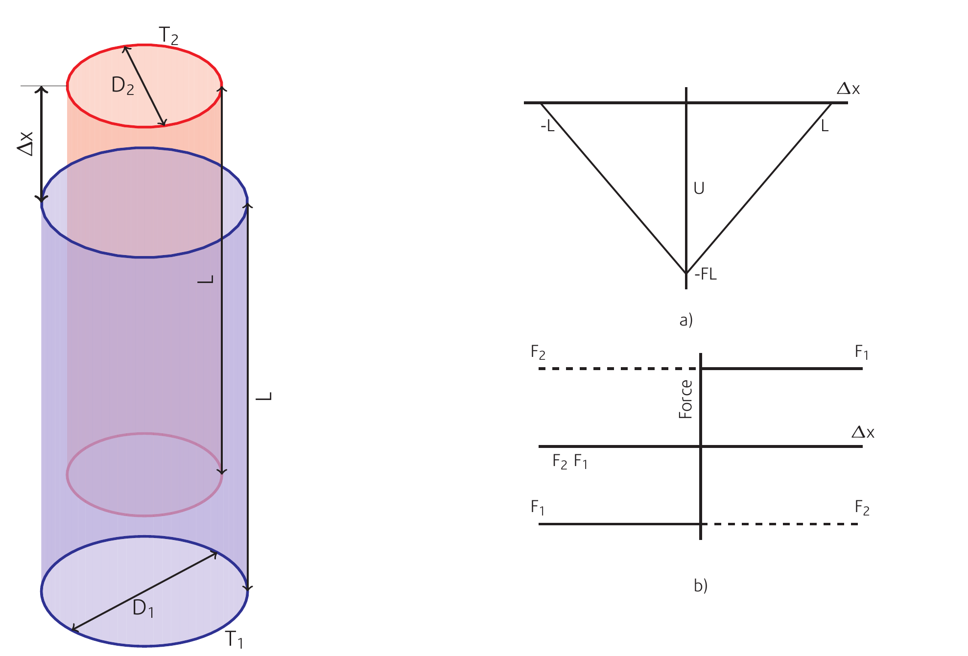
Consider two smooth tubes \(T_1\) and \(T_2\), of length L and diameters \(D_1\) and \(D_2\) as shown in Fig Two telescopic nanotubes , with \(D_1 > D_2\). The diameters are such that \(T_2\) can slide into \(T_1\) telescopically.

The displacement \(Δx\) of one tube with respect to the other is

\[Δx=|x_2-x_1|\]

Where \(x_1\) and \(x_2\) define the locations of the centre of mass of each tube. Note we have defined \(Δx\) so that it is always positive. It is reasonable to assume that the interaction energy U between the two tubes is proportional to the length of the overlap between them. Thus

\[U(∆x)=F(∆x-L)\]

where F is a constant, which has the units of force. Notice that when \(Δx=0\), \(U(Δx)=-FL\), which corresponds to the minimum energy. Also when \(Δx=L\), \(U(Δx)=0\), as you would expect, since the tubes are then fully withdrawn from each other. A plot of the system energy is shown in a), which is plotted as a function of \(x_2-x_1\) to show that the inner tube may extend in the negative direction as well as the positive. The forces acting on the tubes are obtained from the (negative) derivative of the energy, from which we have:

\[\begin{split}\begin{split} F_1 = &+F\; and\; F_2 = -F\; when\; x_2-x_1 > 0 \\ F_1 = &-F\; and\; F_2 = +F\; when\; x_2-x_1 < 0 \end{split}\end{split}\]

which is plotted in , b). So, when the inner tube \(T_2\) is displaced in the positive direction, it experiences a constant force -F pulling in the negative direction, and when it is displaced in the negative direction it experiences a constant +F force pulling it in the positive direction. The opposite is true for the outer tube \(T_1\). This pattern of forces implies an oscillatory system.

Mathematical Exercise

Assuming the system starts from a stationary condition where \(Δx=X_0\), and Newton’s Laws of Motion, derive formulae expressing the position of each tube as a function of time, neglecting any possible friction. You may assume that the tubes have masses \(M_1\) and \(M_2\) and that when \(Δx=0\), then \(x_1=x_2=0\) (i.e. this corresponds to the system centre of mass). Then use the model to answer the following queries:

1. Derive a formula for the period of oscillation of the system in terms of the parameters of the model.

2. The forces do not represent simple harmonic motion in this case, in what ways is it different?

3. How can we use the formula derived for the period of oscillation to determine the important parameter F?

Try to work these out before seeing the solution, see subsection [sec:solution]. When you have answered these queries, you will be ready to tackle the molecular dynamics simulation.

Task

1. Copy or download the following files: CONFIG FIELD CONTROL and run the simulation.

2. Visualise the initial and final configurations using the CONFIG and REVCON files to see if it has evolved to a sensible structure. Use a program such as VMD to view an overview of the whole simulation from the HISTORY file.

3. Write a script to plot the system energies and temperature over time from the STATIS file. Of particular interest is the configuration energy (does this make sense in terms of out model?).

4. See the following sections for a more in-depth numerical analysis of the simulation results.

Analysing the Results

Having amused yourself looking at movies, it’s time to get quantitative. We need to determine the period of oscillation of the system so we can determine the force F in our model. It is hard to do this from the movie! To get a quantitative answer, copy or download the comhis.F90 program and compile using an available Fortran compiler. Use this to calculate the position of the centre of mass of the inner tube \(T_2\), using data in the HISTORY file and plot it as a function of time. The output file is called COM.XY.

gfortran -O3 -o comhis comhis.F90

The command to execute the program is simply: comhis noOfAtoms, where noOfAtoms is the number of atoms in the outer tube, \(T_1\).

From such a plot you should be able to estimate the period of oscillation with fair accuracy. It is also necessary to determine the sweep of the oscillation – how far the tube moves between stationary points on the plot. Both are needed to calculate the force F. Another way to determine the period of oscillation is to Fourier transform the plot of the centre of mass motion. This will project out of the data the true frequency of oscillation, which is the reciprocal of the period. Unfortunately, this is not as trivial as it sounds, so we have provided the program fft.f.

gfortran -O3 -o fft fft.f

Use this to obtain the Fourier transform of the file COM.XY and plot the output file FFT.XY. Use the command:

fft < COM.XY > FFT.XY

Determine the frequency of the oscillation and from it, the period. How does this compare with your previous determination?

Those of you who have a particular interest in using Fourier transforms for frequency analysis should look at the program fft.f and see how this works. Don’t worry about the FFT subroutine itself; this is normally a ‘black box’ routine from a numerical library. Look instead at:

• The subtraction of the mean value of the input function before the Fourier transform is done;

• The way the Dirichlet boundary conditions are applied to the first and last points of the input data; and

• The use made of a window function – in this case a Gaussian.

These tricks are often neglected in naive applications of FFTs, and the result is a confusing, noisy function. Note also that fft.f calculates the modulus of the (complex) Fourier transform, since we are interested only in the amplitude, and not the phase of the oscillation.

Key question: Using the information gathered above what is your estimate of the force constant F in our mathematical model? If you have time, try to do at least one more simulation, using a different diameter for the outer tube \(T_1\).

Further Investigations

You should already have seen how the system configuration energy compares with the mathematical model, but what about the force? The model says this should be constant either side of the origin of the coordinates, but switch sign as we pass through the origin. How can we verify these? We can use the Verlet algorithm!

The standard Verlet algorithm is:

\[x_{n+1}=x_{n-1} + Δt^2 F_n/M\]

which is easily rearranged to:

\[F_n = M(x_{n+1} - 2x_n + x_{n-1}) / Δt^2\]

So we see that we may perform a numerical differentiation of the position of the tube with respect to time to obtain the force.

We have provided the program acceln.f, which uses this approach to calculate the acceleration of a tube, using the data in the file COM.XY. Compile the program and run it using the commands:

gfortran -O3 -o acceln acceln.f
acceln < COM.XY > ACC.XY.

Now plot the file ACC.XY. How well does this result compare with the model? In what ways is it different and why?

We have made no mention of friction in this treatment. How could you go about determining the effect of this? Devise an experiment that you could do to test this. Speculate on the effect that temperature might have on the simulation. Would it increase or decrease friction?

Now you’ve done at least one simulation and seen at least one movie, you should think about how the experiment can be improved. Did anything unexpected happen? Would this affect the validity of our simple model? How would you amend the model to make it more consistent with the simulation?

Some example results

A sample of results are presented in

Sample results

\(T_2\)	Frequency [\(ps^{-1}\)]	Period [ps]	\(X_0\) [Å]	m [D]	Force [\(DAps^{-2}\)]
16	0.0915	10.93	8.085	138.67	300.3
17	0.0831	12.04	9.390	141.44	293.2
18	0.0864	11.57	9.935	144.00	342.0
19	0.0729	13.72	9.300	146.37	231.4
20	0.0661	15.13	8.900	148.57	184.8
21	0.0746	13.41	9.505	150.62	254.8

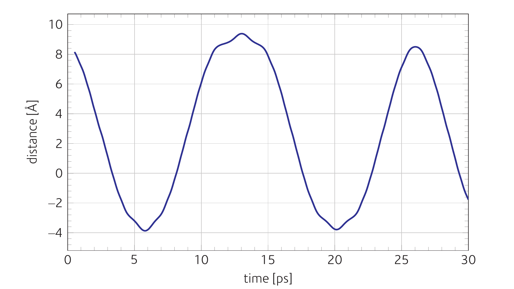
Centre of mass movement

Sample graph of center of mass movement in fig Centre of mass movement and a sample video can be seen on youtube at https://youtu.be/S6q2dr-p5DU.

Solution

The potential energy is:

\[U=F(∆x-L)\]

and the derivatives w.r.t. \(x_1\) and \(x_2\) (i.e. the forces) are:

\[\begin{split}\begin{split} -\frac{dU}{dx_1} &= sgn(x_2 - x_1) F \\ -\frac{dU}{dx_2} &= - sgn(x_2 - x_1) F. \end{split}\end{split}\]

So the equations of motion are:

\[\begin{split}\begin{split} M_1\frac{dv_1}{dt} &= sgn(x_2 - x_1) F \\ M_2\frac{dv_2}{dt} &= - sgn(x_2 - x_1) F \end{split}\end{split}\]

Integrating w.r.t. time gives:

\[\begin{split}\begin{split} M_1v_1 &= sgn(x_2 - x_1) Ft \\ M_2v_2 &= - sgn(x_2 - x_1) Ft \end{split}\end{split}\]

In which the integration constants are zero, for a stationary start. This however cannot be the whole story. We see clearly from , b) that there is a discontinuity in the force when \(x_2-x_1\) changes sign. This means that the integration over time must be performed piecewise, with each piece being evaluated between the discontinuities. For now however, we shall integrate from the time t=0 to the first instance when \(x_2-x_1\) changes sign. This will be sufficient for our needs. Integrating w.r.t. time a second time (subject to the condition \(x_2 - x_1 > 0\)) gives:

\[\begin{split}\begin{split} M_1x_1 &= sgn(x_2 - x_1) Ft^2/2 - C \\ M_2x_2 &= - sgn(x_2 - x_1) Ft^2/2 + C \end{split}\end{split}\]

Where, following from the fact that the centre of mass of the system is at the origin, and using the initial displacement \(X_0\), we have:

\[C = \frac{M_1M_2X_0}{M_1+M_2} \; or\; C = mX_0.\]

Concentrating now on the inner tube \(T_2\), we see that when t=0, the position of the tube is given as \(x_2 = C/M_2\), which is positive. At the same time \(x_1\) is negative, so the sign of \(x_2 – x_1\) is positive. Thus as t increases, \(x_2\) must decrease. In fact the fomulae above show that the change in \(x_2\) is quadratic in time and resembles a free falling object under gravity. At the point \(x_2 = x_1\), the force switches sign but retains its magnitude, so the motion thereafter will be the exact opposite of what has happened until now (replace \(x_2\) with \(-x_2\), \(v_2\) with \(–v_2\), F with –F), it will be a deceleration that carries the tube \(T_2\) to the point \(–C/M_2\). The motion from there on retraces the whole sequence so far and an oscillation is therefore established. In the first part of the motion, the time taken for \(T_2\) to ‘fall’ from position \(x_2=C/M_2\) to \(x_2=0\) is given by:

\[0 = -Ft^2/2 + C \; i.e. \; t = \sqrt{\frac{2C}{F}}\]

This represent one quarter of a full oscillation, so the period of oscillation \(t_2\) of tube \(T_2\) is given by:

\[t_2 = \sqrt{4\frac{2C}{F}}\]

Note that the period of the oscillation depends on the magnitude of C i.e. on the initial displacement of the tubes. This is different from simple harmonic motion, in which the period is independent of the initial displacement. Another way in which the motion differs from SHM, is that it is piecewise quadratic in time, so it does not follow a simple trigonometric function [e.g. \(x_2 = A sin(t/t_2)\)]. To determine the force constant F, we can simply invert the above formula and obtain

\[F = \frac{32C}{t_2^2}\; or\; F = 32 m \frac{X_0}{t_2^2}\]

We can obtain \(X_0\) conveniently by noting that the sweep of the oscillation (i.e. the distance travelled from one stationary point to another – from one peak of the plot to the next trough) is \(2X_0\).

Zheng2002

17. Zheng, J. Z. Liu, and Q. Jiang, Excess van der Waals interaction energy of a multiwalled carbon nanotube with an extruded core and the induced core oscillation, Phys. Rev. B, 65, p. 245409, May 2002, doi: 10.1103/PhysRevB.65.245409

Rivera2003

10. 12. Rivera, C. McCabe, and P. T. Cummings, Oscillatory behavior of double-walled nanotubes under extension: a simple nanoscale damped spring, Nano Letters, 3(8), p. 1001, 2003, doi: 10.1021/nl034171o

Rivera2005

10. 12. Rivera, C. McCabe, and P. T. Cummings, The oscillatory damped behaviour of incommensurate double-walled carbon nanotubes, Nanotechnology, 16(2), p. 186, 2005, doi: 10.1088/0957-4484/16/2/003